Download
1 / 35
350 likes | 517 Vues
Chapter Seven Introduction to Sampling Distributions Section 2 The Central Limit Theorem. Key Points 7.2. For a normal distribution, use mu and sigma to construct the theoretical sampling distribution for the statistic x – bar

E N D
Chapter Seven Introduction to Sampling Distributions Section 2 The Central Limit Theorem
Key Points 7.2 • For a normal distribution, use mu and sigma to construct the theoretical sampling distribution for the statistic x – bar • For large samples, use sample estimates to construct a good approximate sampling distribution for the statistic x-bar • Learn the statement and underlying mean of the central limit theorem well enough to explain it to a friend who is intelligent, but (unfortunately) does not know much about statistics
Let x be a random variable with a normal distribution with mean and standard deviation . Let be the sample mean corresponding to random samples of size n taken from the distribution.
Facts about sampling distribution of the mean: • The distribution is a normal distribution. • The mean of the distribution is (the same mean as the original distribution). • The standard deviation of the distribution is (the standard deviation of the original distribution, divided by the square root of the sample size).
We can use this theorem to draw conclusions about means of samples taken from normal distributions. If the original distribution is normal, then the sampling distribution will be normal.
The mean of the sampling distribution is equal to the mean of the original distribution.
The standard deviation of the sampling distribution is equal to the standard deviation of the original distribution divided by the square root of the sample size.
The time it takes to drive between cities A and B is normally distributed with a mean of 14 minutes and a standard deviation of 2.2 minutes. • Find the probability that a trip between the cities takes more than 15 minutes. • Find the probability that mean time of nine trips between the cities is more than 15 minutes.
Find this area 14 15 Mean = 14 minutes, standard deviation = 2.2 minutes • Find the probability that a trip between the cities takes more than 15 minutes.
Mean = 14 minutes, standard deviation = 2.2 minutes • Find the probability that mean time of nine trips between the cities is more than 15 minutes.
Find this area 14 15 Mean = 14 minutes, standard deviation = 2.2 minutes • Find the probability that mean time of nine trips between the cities is more than 15 minutes.
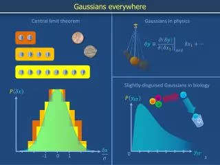
What if the Original Distribution Is Not Normal? Use the Central Limit Theorem!
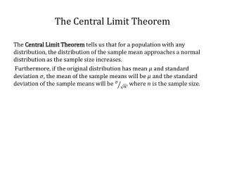
Central Limit Theorem If x has any distribution with mean and standard deviation , then the sample mean based on a random sample of size n will have a distribution that approaches the normal distribution (with mean and standard deviation divided by the square root of n) as n increases without bound.
How large should the sample size be to permit the application of the Central Limit Theorem? In most cases a sample size of n = 30 or more assures that the distribution will be approximately normal and the theorem will apply.
Central Limit Theorem • For most x distributions, if we use a sample size of 30 or larger, the distribution will be approximately normal.
Central Limit Theorem • The mean of the sampling distribution is the same as the mean of the original distribution. • The standard deviation of the sampling distribution is equal to the standard deviation of the original distribution divided by the square root of the sample size.
Application of the Central Limit Theorem Records indicate that the packages shipped by a certain trucking company have a mean weight of 510 pounds and a standard deviation of 90 pounds. One hundred packages are being shipped today. What is the probability that their mean weight will be: a. more than 530 pounds? b. less than 500 pounds? c. between 495 and 515 pounds?
Are we authorized to use the Normal Distribution? Yes, we are attempting to draw conclusions about means of large samples.
Applying the Central Limit Theorem What is the probability that their mean weight will be more than 530 pounds? Consider the distribution of sample means: P( x > 530): z = 530 – 510 = 20 = 2.22 9 9 P(z > 2.22) = _______ .0132
Applying the Central Limit Theorem What is the probability that their mean weight will be less than 500 pounds? P( x < 500): z = 500 – 510 = –10 = – 1.11 9 9 P(z < – 1.11) = _______ .1335
Applying the Central Limit Theorem What is the probability that their mean weight will be between 495 and 515 pounds? P(495 < x < 515) : for 495: z = 495 – 510 = 15 = 1.67 9 9 for 515: z = 515 – 510 = 5 = 0.56 9 9 P( 1.67 < z < 0.56) = _______ .6648