Translating LTL to Automata: State Formulas and Construction Techniques
130 likes | 231 Vues
This chapter delves into converting Linear Temporal Logic to automata, defining state operations and transitions based on current and incoming configurations. It explores various automaton constructions, acceptance sets, and complexity analysis of LTL formulas. Strategies like BDDs and partial order reduction are discussed to mitigate state space explosion issues.

Translating LTL to Automata: State Formulas and Construction Techniques
E N D
Presentation Transcript
Translating LTL to Automata Literature: Peled ch. 6.8 – end of 6 Mads Dam
Automaton State Already processed formulas Previous state identifier Name: Incoming Formulas to be processed New: Old: Formulas for next state Next: Initial nodes: Final nodes = automaton states: Name: Name: Incoming Incoming New: Old: ; New:; Old:1,...,n Next:; Next:1,...,m
Positive Form Positive form: Negation only on primitive state assertions: ::= | : | Æ | Ç | U | V | O Rewriting procedure: ::) :(Æ) ) :Ç: :(Ç) ) :Æ: :( U ) ) (:) V (:) :( V ) ) (:) U (:) :(O) ) O: <>) true U []) false V Rule of substitutivity: ) C[] ) C[] Context C[]: Formula (term) with a “hole” []
Base Step Name Current configuration: Incoming: A New: 1 Old:2 Next:3 Condition: 1 = ; (all formulas have been processed) Is there node Name’ with identical Old, Next? - Then discard Name and add Name.Incoming to Name’.Incoming Otherwise: - Name is a new state - Create new name and node: Name’ Incoming: {Name} New: 3 Old:; Next:;
Case: Proposition Symbol Name Is : 2 2? Yes: Discard the node No: Next configuration: Case for : in New is similar Current configuration: Incoming: A New: , 1 Old:2 Next:3 Name Incoming: A New: 1 Old:, 2 Next:3
Case: Conjunction Name Next configuration: Current configuration: Incoming: A New: Æ , 1 Old:2 Next:3 Name Incoming: A New: ,,1 Old: Æ ,2 Next:3
Case: Disjunction Name Configuration split into two: Current configuration: Incoming: A New: Ç, 1 Old:2 Next:3 Name’ Name’’ Incoming: A Incoming: A New: ,1 Old: Ç , 2 New: ,1 Old: Ç , 2 Next:3 Next:3
Case: Until Name Configuration split into two: Current configuration: Incoming: A New: U , 1 Old:2 Next:3 Name’ Name’’ Incoming: A Incoming: A New: , 1 Old: U , 2 New: , 1 Old: U , 2 Next:3 Next: U , 3
Case: Release Name Configuration split into two: Current configuration: Incoming: A New: V , 1 Old:2 Next:3 Name’ Name’’ Incoming: A Incoming: A New: , , 1 Old: V , 2 New: , 1 Old: V , 2 Next:3 Next: V , 3
Case: Next Name Next configuration: Current configuration: Incoming: A New: O, 1 Old:2 Next:3 Name Incoming: A New: 1 Old: O, 2 Next:, 3
Constructing the Automaton Automaton: (Q,,,I,F) • = truth assignments of propositional symbols in Ex: {a, b, : c, : d} 2 • Q = {final nodes} = {q | q.New = ;} • = {(q,,q’) | q.Name2 q’.Incoming and { | 2 q’.Old} µ and {: | : 2 q’.Old} µ} • I = {q}, q special initial node to kick off construction • Generalized Buchi automaton acceptance set F = {f1,...,fn}: Each fi determined by subformula of shape i U i fi = {q | either i2 q.Old or i U i q.Old}
Complexity Let be given LTL formula Size of state is O(||) Size of automaton is O(2||) Alternative construction can be given such that • States can be recognized in poly time and space • Transitions can be recognised in poly time and space Then complexity of deciding satisfaction is • Polynomial for Buchi automata • (use a binary search procedure) • PSPACE complete for LTL • NONELEMENTARY for monadic 2nd order logic But keep in mind the state space explosion problem!
State Space Explosion |Global state space|: exponential in number of component processes Strategies: BDD’s: • Symbolic representation of states, as DAG’s Partial order reduction: • Recognise states reached by different interleavings • Symmetry reductions a a b b => a b b a =
![LTL Properties B ü chi automata [Vardi and Wolper LICS 86]](https://cdn1.slideserve.com/1829837/cs-267-automated-verification-lecture-8-automata-theoretic-model-checking-instructor-tevfik-bultan-dt.jpg)