Download
1 / 51
510 likes | 726 Vues
Video Traffic Modeling Using Seasonal ARIMA Models. Abdel-Karim Al-Tamimi and Raj Jain Washington University in Saint Louis Saint Louis, MO 63130 Jain@cse.wustl.edu These slides are available on-line at: http://www.cse.wustl.edu/~jain/wimax/video82.htm. Overview. Video Compression overview

E N D
Video Traffic ModelingUsing Seasonal ARIMA Models Abdel-Karim Al-Tamimi and Raj JainWashington University in Saint LouisSaint Louis, MO 63130Jain@cse.wustl.edu These slides are available on-line at: http://www.cse.wustl.edu/~jain/wimax/video82.htm
Overview • Video Compression overview • Seasonal ARIMA Model • Model for all frames combined • Models for I, P, B frames
Goals • One approach to model video traffic is to just determine the distribution of the frame sizes • This assumes that the traffic is white noise and there is no predictability • If there is predictability, it can be used for resource management • Predictability Þ Correlation in frame sizes • In video traffic, there is significant correlation. If a particular scene takes place in a complex background Þ Large frame sizes through out the scene • Similarly, if the scene is simple, the frame sizes will remain low through out the scene.
I I I P P I B P B I B P B I A Typical Group Of Pictures (GOP) I B B P B B P B B P B B P B B I Transmission Order of a GOP I P B B P B B P B B P B B I B B Group of Pictures
Video Scene is divided into group of pictures (GOP) The default GOP size for NTSC: 15 GOP consists of: I (Intracoded) frames: Each frame of video is still discrete and can be accessed as a unique point P (Predicted) frames: P frames are predicted based on prior I or P frames B (bi-directional predicted) frames: B frames are coded based on a forward prediction from a previous I or P frame, as well as a backward prediction from a succeeding I or P frame MPEG Encoding
Video Trace • Using ffmpeg library, we encoded 1:24 minutes movie clip • At 350kbps • QVGA: 320x240 • GOP size of 15 • GOP sequence is : • IBBPBBPBBPBBPBB
Video Frames: A Closer Look • Observation: Every 15th frame is a large (I) frame. I Frames
Video Frames: I, P, B Size Distribution • Observation: I, P, B frames have very different levels. I-frames P-Frames B-Frames
Auto-Regressive Models • AR(1) Model: y(t) = a(1) y(t-1) + w(t) • AR(p) Model: y(t) = a(1) y(t-1) + a(2)y(t-2)+…+a(p)y(t-p)+w(t) • AR(0) Model: y(t)=w(t) Þ White noise • Auto-Correlation Function (ACF): AC(k)=cov(Y(t),y(t-k))/Var(y(t)) • Partial Auto-Correlation Function (PACF): PACF cuts off at p for AR(p) a0 a1 a2 PACF(k) a3 ACF(k) 0 1 2 3 4 5 0 1 2 3 Lag k Lag k
Moving Average Models • MA(1) Model: y(t) = w(t)+b(1) w(t-1) • MA(q) Model: y(t) = w(t)+b(1) w(t-1) + b(2)w(t-2)+…+b(q)w(t-q) • MA(0) Model: Y(t)=w(t) Þ White noise b0 ACF cuts off at q for MA(q) b1 b2 b3 PACF(k) ACF(k) 0 1 2 3 0 1 2 3 3 3 3 Lag k Lag k
ARIMA Models • ARMA(p,q) Model: y(t) + a(1)y(t-1)+…+a(p)y(p) = w(t)+b(1) w(t-1)+…+b(q)w(t-q) • Using Backward operator: Dy(t)= y(t-1) {1+a(1)D+a(2)D2+…+a(p)Dp}y(p)={1+b(1)D+…+b(q)Dq}w(t) A(D)y(p) = B(D)w(t) • Auto-regressive Integrated Moving Average Model: ARIMA(p,d,q) A(D)(1-D)dy(p) = B(D)w(t) • Example: ARIMA(1,1,1) Model (1+a1D)(1-D)y(t)=(1+b1D)w(t) (1+a1D-D-a1D2)y(t) = (1+b1D)w(t) y(t)-(1-a1)y(t-1)-a1y(t-2)=w(t)+b1w(t-1)
Seasonal ARIMA Model • Period of 12 Þ Model y(t)-y(t-12) as a ARIMA(p,d,q) series • ACF will show spikes at seasonal period s • Seasonal ARIMA(p,d,q) (P,R,Q)s model: A(D)F(Ds)(1-Ds)Ry(t)=B(D) G(Ds)w(t) • Example: (1,0,0)x(0,1,0)12 Model (1+a1D)(1-D12)y(t)=w(t) y(t)-y(t-12)-a(1){y(t-1)-y(t-13)}=w(t) y(t) JFMAMJJASOND JFMAMJJASOND JFMAMJJASOND Month t
Interpreting ACF and PACF ] : Time Series Analysis and Its Applications: With R Examples Trails off at lag = 1 OR cuts of at lag = 2
ACF (Auto-Correlation Function) graph shows many trends and show how much video frames are correlated Traffic Modeling – All Frames 1
A closer look at the ACF graph shows a strong continual correlation every 15 lag GOP size Traffic Modeling – All Frames 2
ACF graph after second level of differentiation with seasonal part of 15 Traffic Modeling – All Frames 3
PACF (Partial Auto-Correlation Function) shows another decaying trend around lags 15,30,45 . Also around 14,29,44 Traffic Modeling – All Frames 4
Traffic Modeling – All Frames 5 -Within the same seasonal part : cuts off/trails at h=1 , (ignore at lag 14) -Across seasonal parts : trails at h=1
Traffic Modeling – All Frames 6 -Within the same seasonal part : trails at h=1 -Across seasonal parts : trails at h=1
The chosen seasonal ARIMA model is: (1,1,1) x (1,1,1)15 Coefficients : Traffic Modeling – All Frames 7
Results 2 Blue : Fitted Model Red : Original data R2 = 0.88
The chosen seasonal ARIMA model is: (1,1,1) x (1,1,1)15 Coefficients : Modeling All Frames: Seasonal ARIMA Model
Modeling All Frames: Log Seasonal Model Blue : Fitted Model Red : Original data R2 = 0.99
Modeling I, P, B Frames Separately • Another approach to consider while modeling video traffic is to separate the three video frame types as individual models • Create separate models for I-Frames, P-Frames and B-Frames • Compare the final results with the one obtained from the previous approach
Modeling I Frames 2 Only one correlation at lag = 1 ignore
Modeling I Frames 3 Only one correlation at lag = 1 ignore
The Proposed models are: ARIMA(0,0,1), ARIMA(1,0,0), ARIMA(1,0,1) Determine the best model based on AIC (Akaike's Information Criterion) AIC = 2k –2 ln L = 2k + n[ln(2p RSS/n) + 1]Here k is the number of parameters and L is the “goodness of the model” RSS = Residual sum of squares Lower AIC Þ Smaller number of parameters and lower errors Akaike’s Information Criterion (AIC) [1] : http://en.wikipedia.org/wiki/Akaike_information_criterion
Proposed models : ARIMA(0,0,1), ARIMA(1,0,0), ARIMA(1,0,1) Now we determine the best model based on AIC index (lower is better) ARIMA(0,0,1) [AIC] = 1922.87 ARIMA(1,0,0) [AIC] = 1913.42 √ ARIMA(1,0,1) [AIC] = 1913.82 Modeling I Frames 4
Modeling I Frames 6 • Coefficients:
Modeling I Frames: Results Blue : Fitted Model Red : Original data R2 = 0.98
Modeling P Frames 2 Trails off at lag = 1 ignore
Modeling P Frames 3 Trails off at lag = 1 ignore cuts off at lag = 2
Modeling P Frames 4 • ACF : Trails off at lag =1 • PACF : Trails off at lag =1, cuts off at lag =2 • ARIMA models • ARIMA(1,0,1) AIC = 7724.41 √ • ARIMA(2,0,0) AIC = 7733.21 • Model coefficients:
Modeling P Frames 6 Blue : Fitted Model Red : Original data R2 = 0.81
Modeling B Frames 2 ignore
Modeling B Frames 2 Trails off at lag = 1
Modeling B Frames 3 Trails off at lag = 1 Cuts off or Trails off at lag = 5 ignore
Modeling B Frames 4 • ARIMA Models • ARIMA(1,0,1) AIC = 15315.06 • ARIMA(5,0,0) AIC = 15187.51 • ARIMA(5,0,1) AIC = 15186.66 √
Modeling B Frames 6 Blue : Fitted Model Red : Original data R2 = 0.89
Combining I, P, B Models 1 • To get a full model for all frames, a combination of the model will be presented. • Points to consider: • The three models represented for I-Frames, P-Frames and B-Frames did not show the seasonal trend • Models are easier to implement than the All-Frames models
Combining I, P, B Models 2 Blue : Fitted Model Red : Original data R2 = 0.82
Summary • In this presentation we showed that a good model for video traffic is achievable using ARIMA model • Seasonal ARIMA is a better approach to get a better video traffic model • Creating individual models for each frame type is not necessary a better approach