Download
1 / 17
180 likes | 425 Vues
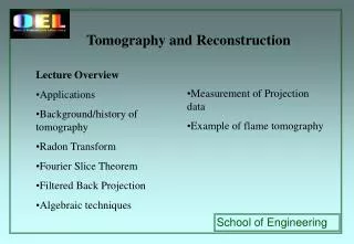
Tomography and Reconstruction. Lecture Overview Applications Background/history of tomography Radon Transform Fourier Slice Theorem Filtered Back Projection Algebraic techniques. Measurement of Projection data Example of flame tomography. Applications & Types of Tomography.

E N D
Tomography and Reconstruction • Lecture Overview • Applications • Background/history of tomography • Radon Transform • Fourier Slice Theorem • Filtered Back Projection • Algebraic techniques • Measurement of Projection data • Example of flame tomography
Applications & Types of Tomography MRI and PET showing lesions in the brain. PET scan on the brain showing Parkinson’s Disease
Applications & Types of Tomography ECT on industrial pipe flows
The History • Johan Radon (1917) showed how a reconstruction from projections was possible. • Cormack (1963,1964) introduced Fourier transforms into the reconstruction algorithms. • Hounsfield (1972) invented the X-ray Computer scanner for medical work, (which Cormack and Hounsfield shared a Nobel prize). • EMI Ltd (1971) announced development of the EMI scanner which combined X-ray measurements and sophisticated algorithms solved by digital computers.
The function is known as the Radon transform of the function f(x,y). Line Integrals and Projections
Line Integrals and Projections A projection is formed by combining a set of line integrals. Here the simplest projection, a collection of parallel ray integrals i.e constant θ, is shown. A simple diagram showing the fan beam projection
Fourier Slice Theorem The Fourier slice theorem is derived by taking the one-dimensional Fourier transform of a parallel projection and noting that it is equal to a slice of the two-dimensional Fourier transform of the original object. It follows that given the projection data, it should then be possible to estimate the object by simply performing the 2D inverse Fourier transform. Start by defining the 2D Fourier transform of the object function as The part in brackets is the equation for a projection along lines of constant x Define the projection at angle θ, Pθ(t) and its transform by Substituting in For simplicity θ=0 which leads to v=0 Thus the following relationship between the vertical projection and the 2D transform of the object function: As the phase factor is no-longer dependent on y, the integral can be split.
v v u u The Fourier Slice Theorem The Fourier Slice theorem relates the Fourier transform of the object along a radial line. Collection of projections of an object at a number of angles t Fourier transform θ For the reconstruction to be made it is common to determine the values onto a square grid by linear interpolation from the radial points. But for high frequencies the points are further apart resulting in image degradation. Space Domain Frequency Domain
Filtered Back Projection Filtered back projection is the most commonly used algorithm for straight ray tomography. The result of back projecting (a)The ideal Situation (b) Fourier Slice Theorem (c) The filter back projection takes the Fourier Slice and applies a weighting so that it becomes an approximation of that in (a).
Figure b. The indeterminate problem. Figure a. Initial 3 by 3 grid with ray sums and coefficients. Figure c. Step 1: All entries in unity, scaled by ray sum over number of row elements. Figure e. Step 3. Recalculated row and column sums and elements. Figure d. Step 2: Recalculated column sums. Σx Σx Σx Σx Σx 6 6 6 6 6.01 ? 6/3 1.5 6/3 1 1.88 3 6/3 6/3 ? 6/3 6/3 2 ? 2.63 1.25 1 5/3 5/3 ? 5/3 ? 5/3 1.57 1 5/3 ? 2.19 5/3 3 5 5 5 5 5.01 5/3 5/3 2 1.25 ? ? 1 5/3 1.57 5/3 ? 5/3 5/3 2.19 2 5 5 5 5 5.01 4 4 4 4 5.33 5 5 5.02 5 5.33 7 5.33 7 7 7.01 Σy Σy Σy Σy Σy The Array: Algebraic Reconstruction Technique (ART) ART is used in indeterminate problems and was first used by Gordon et al in the reconstruction of biological material.
Measurement of projection data Attenuation of X-rays Assume no loss of intensity of the beam due to divergence, however the beam does attenuate due to photons either being absorbed or scattered by the object. Photoelectric Absorption This consists of an x-ray photon imparting all of its energy to an inner electron of an atom. The electron uses this energy to overcome the binding energy within its shell, and the rest appearing as kinetic energy in this freed electron. Compton Scattering This consists of the interaction of the photon with either the free electron or a loosely bound outer shell electron. As a result the x-ray is deflected from its original direction.
Measurement of projection data Attenuation of X-rays Solving this across the thickness of the slab Consider N photons cross the lower boundary of this layer in some measured time interval, and N+ΔN emerge from the top side. (ΔN will be negative). ΔN follows the relationship, Where N0 is the number of photons that enter the object. The number of photons as a function of the position within the slab is given by, μ=photon loss rate (per unit distance) of the Compton and photoelectric effects. In the limit Δx goes to zero so we get or
Background Lamp, L1 Flame, L3 Flame+Lamp, L Counts 77.71 93.76 439.29 450.82 Minus Background - 16.06 361.59 373.12 Fibre optic to spectrograph Mercury lamp Transmitted portion of back light radiation, L2 Burner Radiant intensity of backlight, L1 Radiance emitted by gas, L3 Signal enteringflame Signal leaving flame Optical arrangement used to determine the optical thickness of a flame. Flame Thickness, Emission and Absorption Interpretation of Results Transmitted portion of backlight radiation, L2: 11.53 counts Radiation incident on fibre from backlight, L1: 16.06 counts 72% transmission at 309 nm Optical thickness at 309 nm, Absorption Coefficient: Emission Coefficient:
Tomographic array Fibre optic 3.8 Acceptance cone of fibre The acceptance cone of the fibres fitted to the area The Array: Fibre Geometry
Averaged thermocouple result Single Photograph of OH modified for colour intensity Single thermocouple scan Average of three photographs Comparing Results The burner has been modified by placing two coins on it’s base. The array result is shown, superimposed on a photograph of the modified burner.