Signal Flow Graphs
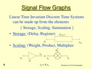
T or z -1. A. y k. or. y k. x k. x k. A. x k. x k -1. y k = A.x k. Signal Flow Graphs. Linear Time Invariant Discrete Time Systems can be made up from the elements { Storage, Scaling, Summation } Storage: (Delay, Register) Scaling: (Weight, Product, Multiplier. +. X + Y.

Signal Flow Graphs
E N D
Presentation Transcript
Tor z-1 A yk or yk xk xk A xk xk-1 yk= A.xk Signal Flow Graphs Linear Time Invariant Discrete Time Systems can be made up from the elements { Storage, Scaling, Summation } • Storage: (Delay, Register) • Scaling: (Weight, Product, Multiplier 1
+ X + Y X + Y Signal Flow Graphs • Summation: (Adder, Accumulator) • A linear system equation of the type considered so far, can be represented in terms of an interconnection of these elements • Conversely the system equation may be obtained from the interconnected components (structure). 2
b yk xk z-1 yk-1 a1 yk-2 a2 Signal Flow Graphs • For example 3
Signal Flow Graphs • A SFG structure indicates the way through which the operations are to be carried out in an implementation. • In a LTID system, a structure can be: i) computable : (All loops contain delays) ii) non-computable : (Some loops contain no delays) 4
Signal Flow Graphs • Transposition of SFG is the process of reversing the direction of flow on all transmission paths while keeping their transfer functions the same. • This entails: • Multipliers replaced by multipliers of same value • Adders replaced by branching points • Branching points replaced by adders • For a single-input / output SFG the transpose SFG has the same transfer function overall, as the original. 5
Structures • STRUCTURES: (The computational schemes for deriving the input / output relationships.) • For a given transfer function there are many realisation structures. • Each structure has different properties w.r.t. • i) Coefficient sensitivity • ii) Finite register computations 6
Signal Flow Graphs Direct form 1 : Consider the transfer function • So that • Set 7
z-1 z-1 z-1 n delays a0 a1 a2 an + + + + W(z) Signal Flow Graphs • For which • Moreover 8
W(z) Y(z) + + - - - - z-1 b1 z-1 b2 z-1 b3 z-1 bm m delays Signal Flow Graphs • For which 9
Signal Flow Graphs • This figure and the previous one can be combined by cascading to produce overall structure. • Simple structure but NOT used extensively in practice because its performance degrades rapidly due to finite register computation effects 10
Signal Flow Graphs • Canonical form: Let • ie • and 11
+ + a0 a1 a2 Y(z) X(z) + + + + - W(z) an - - b1 b2 bm Signal Flow Graphs • Hence SFG (n > m) 12
Signal Flow Graphs • Direct form 2 : Reduction in effects due to finite register can be achieved by factoring H(z) and cascading structures corresponding to factors • In general with • or 13
Signal Flow Graphs • Parallel form: Let • with Hi(z) as in cascade but a0i = 0 • With Transposition many more structures can be derived. Each will have different performance when implemented with finite precision 14
U(z) V(z) 2 1 3 4 Y(z) X(z) Linear T-I Discrete System Signal Flow Graphs • Sensitivity: Consider the effect of changing a multiplier on the transfer function • Set • With constraint 15
Signal Flow Graphs • Hence And thus 16
X2(z) X1(z) Linear Systems S T(z) Y1(z) Y2(z) Signal Flow Graphs • Two-ports 17
x1(n) y1(n) M x2(n) y2(n) Signal Flow Graphs • Example: Complex Multiplier 18
+ + + x1(n) y1(n) - + x2(n) y2(n) + Signal Flow Graphs • So that • Its SFD can be drawn as 19
Signal Flow Graphs • Special case • We have a rotation of t o by an angle • We can set so that and • This is the basis for designing • i) Oscillators • ii) Discrete Fourier Transforms (see later) • iii) CORDIC operators in SONAR 20
Signal Flow Graphs • Example: Oscillator • Consider and externally impose the constraint So that • For oscillation 21
Signal Flow Graphs • Set • Hence 22
Signal Flow Graphs • With and , the oscillation frequency • Set then and • We obtain • Hence x1(n) and x2(n) correspond to two sinusoidal oscillations at 90 w.r.t. each other 23
+ + + + + + Signal Flow Graphs Alternative SFG with three real multipliers 24
Signal Flow Graphs • Example: Oscillator 25