GHz Differential Signaling
GHz Differential Signaling. High Speed Design . ISI (Inter-Symbol Interference). Frequency dependant loss causes data dependant jitter which is also called inter symbol interference (ISI). In general the frequency dependant loss increase with the length of the channel.

GHz Differential Signaling
E N D
Presentation Transcript
GHz Differential Signaling High Speed Design
ISI (Inter-Symbol Interference) • Frequency dependant loss causes data dependant jitter which is also called inter symbol interference (ISI). • In general the frequency dependant loss increase with the length of the channel. • The high frequencies associated with a fast edge are attenuated greater than those of lower frequencies. • The observable effect on a wave received at the end of a channel looks as if the signal takes time to charge up. If we wait long enough the wave reaches the transmitted voltage. If we don’t wait long enough and a new data transition occurs, the previous bit look attenuated. Hence a stream of bits will start or finish the charge cycle at different voltage point which will look to the observer as varying amplitudes for various bits in the data pattern. Introduction
channel Rx channel Rx channel Rx channel Rx Effect of increasing channel length • Notice the effect on the lone narrow bit verses the wider pulse that is representative of multiple bits. • The lone pulse looks more and more like a runt as the channel length increases Tx Introduction
Simulation of a lossy channel ISI • Example is 1 meter of FR4 at 1GHz • Notice the loss creates the edge to edge jitter and the max voltage is not reached on the runt pulse This is ISI. Rx Tx Rx Introduction
Transition bit How can we fix the runt pulse? • Solution: Boost the amplitude of the first bit. • The means we drive to a higher voltage at the high frequency component and a lesser voltage at lower frequency. Introduction
Equalization • The previous slide illustrates the concept of equalization. • Normally the max current is supplied on the transition bit and reduces on subsequent bits. Thus if we reference to the transition bit to a transmitter this equalization is commonly called “de”-emphasis. If we talk about the a the non-transition bit in reference to a receiver or passive network we might call this “pre”-emphasis. Although the two may be considered the same, the former is used more commonly. Introduction
Equalization Philosophy – First step • Given the channel has a complex loss verses frequency transfer function, Hch(w) • The FFT of an input signal multiplied by the transfer function in the frequency domain is the response of the channel to that input in the frequency domain. tx(t)Tx(w) • If we take the IFFT of the previous cascade response we get the time domain signal of the output of the channel. We talked about this last semester. rx(t)=IFFT(Tx(w)*Hch(w)) Introduction
Equalization Philosophy – The punch line • Given the response of the output:Tx(w)*Hch (w) • Look what happens if we multiply this product by 1/ Hch (w). The result is Tx(w). • The realization of 1/ Hch (w) is called equalization and my be achieved number of ways. • If applied to the transmitter, it is called transmitter equalization. This approximated by the boost we referred to earlier. • If it is applied at the output of the channel, it is called receiver equalization. • If done properly, the results are the same but cost and operation factors may favor one over the other. Introduction
Bitwise equalization conceptualization dB 1/Hch(f) Ideal equalization • Bitwise equalization • Approximation based on bit transitions • More bits may better approximate 1/h(f) 0dB Hch(f) Frequency Introduction
Introducing the terminology “TAP” This is called 2 tap equalization • It becomes clear what a tap is when we look at lone bit (data pattern ~ …0001000000…) Vshelf Commonly the 2 Tap de-emphasis spec in dB and is -20*log(Vshelf/Vswing) Vswing Tap 2 Tap1 Also called cursor. We will explore the whole concept of cursors later Vtap1 Introduction
The lone bit tap spec is different • Taps are normalized so that sum of the cursor tap minus the pre and post cursor taps is equal to 1 with the base equal to zero. The reason will become clear later. • Lets take the last example where de-emphasis is defined as -6 dB. This would correspond to tap1=0.75 and tap2=0.25. These are called tap coefficients. Tap1: This tap is called the cursor base = 0 tap2 Introduction
0.75 0 0 0 0 0 0 1 0 0 0 0 0 0.0 -0.25 0 0 0 0 0 0 1 0 0 0 0 0 0 0 0 0 0 0 1 0 0 0 0 0 0 0 0 0 0 0 1 0 0 0 0 0 S 0 0 0 0 0 0 1 0 0 0 0 0 0 0 0 0 0 0 1 0 0 0 0 0 0 0 0 0 0 0 0 1 1 1 0 0 0 1 1 1 0 0 0 0 0 Bits 0 0 0 0 0 0 0 ¾ ½ ½ -¼ 0 0 ¾ ½ ½ -¼ 0 0 0 0 Value Use superposition to string together a bit pattern out of lone bits with the amplitude of the taps Introduction
We now have a familiar waveform 0 0 0 0 0 0 0 1 1 1 0 0 0 1 1 1 0 0 0 0 0 Bits 0 0 0 0 0 0 0 ¾ ½ ½ -¼ 0 0 ¾ ½ ½ -¼ 0 0 0 0 Value • Observe that Vshelf is ½ and Vswing is 1. • For 2 tap systems we would call this 6dB de-emphasis 20*log(0.5) • 20*log(Vshelf/Vswing) is not a roust and easily expandable specification but common used in the industry and call the transmitter de-emphasis spec, • A more roust way would be to spec tap coefficients which we will take a bit more about later Renormalize to 1 peak to peak: Value-1/4 -¼ -¼ -¼ -¼ -¼ -¼ -¼ ½ ¼ ¼ -½ -¼ -¼ ½ ¼ ¼ -½ -¼ -¼ -¼ -¼ renorm ½ 1 Introduction
Assignment 8: • What are the tap coefficients for 2 tap equalization with de-emphasis specified at 3.5 dB • Draw and label the lone one pulse tap waveform. • If Vswing is 500 millivolts what is Vshelf Introduction
20fF W 100 -> W 5 40k ->2 W 2.5 0k 20fF Passive Continuous Linear Equalizer (CLE) • The passive CLE is a high pass filter. • Low frequency components are attenuated. • The filter can be located anywhere in the channel, and can be made of discrete components, integrated into the silicon, or even built into cables or connectors. Introduction
D D D x k C C C C -1 0 1 2 S y k Rx Discrete Time Linear Equalizer (DLE) • The receive-side DLE works just like the transmitter pre-emphasis circuit. • The only difference is that it samples the incoming analog voltage. • Uses a “sample & hold” circuit at the input, which provides the input signal stream to the FIR. Introduction
Two Examples of Differential Tx Equalization • Discrete-time Transmitter Linear Equalizer (DTLE)* • This is a type of finite impulse response (FIR) filter • http://www.dspguru.com/info/faqs/firfaq.htm • The equalizations operates over the entire bit stream continuum. • Superposition of all preceding bits • An implementation example will follow. • One characteristic of FIR is that input waves eventually emerge at the output • A FIR filter does not have feedback • Transition Bit Equalization with delayed tap current steering (TBE) • Resets on each transition • This is discrete time but not linear because the superposition does not create linearly effect subsequent waveforms. • Hence this is not really a purely theoretically FIR but is often the way may industry standards are implemented and spec’ed. • Common characteristics of bitwise equalization • Current steering based on UI delay • Normally implemented with “current mode logic” CML • Specified in PCI-Express * Bryan Casper April 2003“ISI Analysis with Equalization Introduction
DTLE Dual Current Source Model D=1 bit delay • Cn’s are called tap coefficients • The delayed signal are multiplied by respective Cn’s and summed. • For behavioral simulation the summed signal may be filter to shape the output wave. D D D V Data Stream C0 C1 C2 C3 P P P P S VCCS 1-S Introduction
V D D D Data Stream 0 DTLE Scaled current source model • The Cn’s coefficient are preset into respectively switched in current sources. C3 C0 C1 C2 C4 Introduction
Discrete Transmitter Equalization Characteristics • The goal is to not have any AC current drain. • Current is steered from positive to negative for each tap switching in. • The normalization is to the maximum available current. Hence the tap coefficients are the apportioned switched currents. • Since the max current is normalized to 1 the sum of all taps must equal to 1. • Another way to look at this is that there is an actual total available current for the buffer. The taps just steer the current from one leg to another. All taps “on” corresponds to the sum of the taps equal which equals to 1. Introduction
V V V V Subsequent Bits + - + - De-Emphasis Achieved by Steering Current • Full swing = Both (all) current sources are on for one leg • This correspond to a one or zero logic state. • This is called the primary leg • De-emphasis is achieved by steering current away from primary leg to secondary leg First Bit Transition Introduction
Differential Behavioral Buffer - Review • Switched current source • D+ and D- switching is complementary • CML – Current mode logic • Goal: Maintains constant current draw in high state, low state, and switching. • Power rails are only disturbed during switch due to asymmetry. V D+ Leg(terminal) D- Leg(terminal) D+ Leg(terminal) D- Leg(terminal) V V Introduction
Switch Control from Data Stream • Problem: need to turn off minus boost during plus and visa versa V V V V boost boost + - + - Data Inverted data 2nd class starts here Plus boost minus boost Introduction
TBE: Switch Control from Data Stream • Problem: need to turn off minus boost during plus and visa versa V V V boost boost + - + - Data (D) Inverted data (!D) Plus boost (P) Will show equation in a few slides Minus boost (Pp) 0 to 1 transition Plus boost off (!P) Minus boost off (!Pp) Introduction
TBE: Switch Control from Data Stream • Problem: need to turn off minus boost during plus and visa versa V V V boost boost + - + - Data (D) Inverted data (!D) Plus boost (P) Will show equation in a few slides Minus boost (Pp) 0 to 1 transition Plus boost off (!P) Minus boost off (!Pp) Introduction
TBE currents • The previous slide illustrate the logic that controls the switches. • The remaining tasks is to determine is the two currents. Introduction
Use Vmax and dB shelf spec to define currents Introduction
Multi tap digital linear equalization (FIR) • We will do the same example as before with equalization taps. • One tap will be at 0.75 and the other at 0.25 • We’ve seen before this corresponds to a 6 dB de-emphasis spec D Unity AmplitudeData Stream C1 V C0 P Filter P S VCCS 1-S Behavioral Example Introduction
HSPICE example – tap waves * test_diff_fir_2_src.sp .param ui=400ps tr=50ps wf=1 Imax=16ma Vpulse in 0 pulse 0 1 0 tr tr '5*UI-Tr' '10*UI' Rin in 0 50 .tran 10ps 10ns .probe v(in) v(in2) v(in1) vin(in0) v(outf) v(datap) +v(datan) v(vip) v(vin) v(vdiff) vvcc vcc 0 2 .param c0=.75 c1=.25 c2=0 Ep0 in0 0 vol='C0*v(in)' Ep1 in1x 0 vol='C1*(1-v(in))' Ep2 in2x 0 vol='C2*(1-v(in))' Edp1 in1 0 DELAY in1x 0 TD='UI' Edn2 in2 0 DELAY in2x 0 TD='2*UI • We will use a pulse source that 10*UI to demonstrate the de-emphasis • Three waveform are created in0, in1, and in2 with respective delays of 0, UI, and 2*UI • Even though this case has three taps we will make tap C2 equal to zero. • C0 and C1 are 0.75 and 0.25 respectively Introduction
Now to create current waves • Create sum of tap wave with 2 volt amplitude • The filter cuts the voltage in half producing a 1 volt peak amplitude at “outf” • The voltage at “outf” and its complement are used to create the current waves Esum outs 0 vol='2*(v(in0)+v(in1)+v(in2))' *simple filter profiles current Routs outs outf 50 Routf outf 0 50 Coutf outf 0 1p * create profile current waveforms * that map to the current Gictlp datap 0 cur='imax*abs(v(outf))' Gictln datan 0 cur='imax*abs((1-v(outf)))' Introduction
Now to create current waves *Convenience node Ediff vdiff 0 vol='v(datap)-v(datan)' * buffer termination loads Rp datap 0 50 Rn datan 0 50 * test load mimics a transmission line Rnload datap 0 50 Rpload datan 0 50 .end • Each source is connected to internal loads and external loads. • A node vdiff is created as a convenience to view the differential waveform Introduction
We observe the wave has 6dB De-emphasis 20 * log(400/800) = 6 dB Introduction
Return loss • Return loss is an important parameter for high speed signal transmission • Lets looks at the channel transfer function. • Notice that Gs and GL is a factor determining the amount of signal that is received a the end of channel • For a 1 port device S11 and G are the same. • Lets review what we discuss before that G is called return loss Introduction
Return Loss Specifications • Very often return loss expressed as dB • Also the minus sign may be omitted. • How ever notice that the absolute value of S11 us used. • Two impedances can be represented by the RL spec. Introduction
Example 0f Impedance Spec From RL Introduction
Anatomy of RL for chips • Lets assign some values and examine the resultant return loss. • Transmission line = 1 inch and 110 ohms • Cpad=1pf/0.5pf and Rpad=55 ohms • Lvia_ball= .3 nH and Cvia_ball=.3pF Transmission line, Z0, Length L via_ball Rpad Cvia_ball Cpad Introduction
Pad capacitance is a critical parameter 1pF Capacitor alone 0.5pF Introduction
RL Sufficiency • Little return loss insures good transmission • Moderate return loss may not be sufficient to insure good transmission for some frequencies • Given 1” package trace which is approx 150 ps • Round trip is 300 ps = ½ period of 3.3 GHz • Reflections could make signal at pin look much worse than at pad. Incident @PIN Reflect from pad @PIN signal @PAD signal @PIN Introduction
Unexpected effects of GHz Clocking • Assumption: Jitter at transmitter is translated to the same amount of jitter at the receiver. • We have used this assumption before in time budgets • Not true because of line loss Tx Rx Introduction
Response of narrower pulse New effect at high frequencies:Jitter amplification • The loss of the pulse that is has a decreased pulse width is more than the pulse with the original pulse width Introduction
In summary here a few high frequency and differential topics we touched upon • Clock recovery • Return loss • Common and differential mode signal • Equalization • Inter-symbol interference (ISI) • Current mode logic • The next task is to evaluate a channel’s quality when all these effects are included. In other words what does the worst signal look like and how do we find it? This will be the subject the next class Introduction
![Frequency [GHz]](https://cdn1.slideserve.com/3024092/slide1-dt.jpg)
![Frequency [GHz]](https://cdn3.slideserve.com/6756635/slide1-dt.jpg)