Improved Algorithms for Link-Based Non-tree Clock Network for Skew Variability Reduction
Improved Algorithms for Link-Based Non-tree Clock Network for Skew Variability Reduction. Anand Rajaram † ‡ David Z. Pan † Jiang Hu * † Dept. of ECE, UT-Austin ‡ Texas Instruments, Dallas * Dept. of EE, TAMU. Outline. Introduction Review of link-based non-tree clock network

Improved Algorithms for Link-Based Non-tree Clock Network for Skew Variability Reduction
E N D
Presentation Transcript
Improved Algorithms for Link-Based Non-tree Clock Network for Skew Variability Reduction Anand Rajaram†‡ David Z. Pan† Jiang Hu* † Dept. of ECE, UT-Austin ‡ Texas Instruments, Dallas * Dept. of EE, TAMU
Outline • Introduction • Review of link-based non-tree clock network • Improved algorithms (over [Rajaram et al, DAC’04]) • Rule based algorithm (δ Rule) • Graph theoretical approach (MST-based) • Experimental results • Conclusions
Launch signals T Clock Distribution Network Register Register • Signal transfer coordinated by clock signal • All registers are supplied with clock signal by clock distribution network • Skew = d1 – d2 • Zero skew: d1 = d2 • Useful skew, d1 – d2 = δ12 Dmax 1 2 Catch signals d1 d2 Clock Network
Clocks : Important Considerations & Objectives • One of the biggest & most frequently switching nets • Very sensitive to unwanted skew introduced by PVT • Manufacturing process variations (P) • Power supply voltage noise (V) • Temperature variations (T) • Less clock skew variation a “MUST” for nanometer VLSI designs • Minimizing clock routing wire-length can • Reduce power consumption
Approaches for Reducing Skew Variability • Buffer & wire sizing [Pullela et al., DAC’93; Chung et al., ICCAD’94; Wang et al., ISPD’04] • Variation aware routing [Lin et al., ICCAD’94; Lu et al., ISPD’03] • Non-tree clock networks • McCoy et al., ETC’94; Vandenberghe et al., ICCAD’97; Xue et al., ICCAD’95 • Link based non-tree clock networks [Rajaram et al., DAC’04]
Non-tree: 1-D Spine [Kurd et.al JSSC’01] • 1-D spine • Applied in Intel Pentium processor design • Variations between spines still exists Spines Clock sinks or local sub-networks
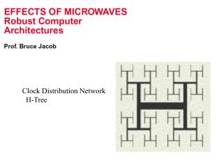
Top level mesh [Su et. al, ICCAD’01] Less wire, less effective Leaf level mesh [Restle et. al, JSSC’01] Very effective, huge wire Applied in IBM microprocessors Non-tree: 2-D Mesh Clock sinks or local sub-networks Clock sinks or local sub-networks
u C/2 Rl w C/2 Rl u w C/2 C/2 Linked Non-tree = Tree + Links[Rajaram et al, DAC’04] • Non-tree = tree + links • How to select link pairs is the key! • Link = link_capacitors + link_resistor i u w
New skew with link (u, w): u Rlink Rloop w • Value of becomes smaller when link is closer to leaf nodes for a given Rlink Skew Between Link Endpoints
Skew Between any Two Nodes (i, j) with Link (u, w) Skew variation between any node pair (i, j) • Scenario1: i Tg , j Th => always smaller • Scenario2: i & j Tg (or Th) => could be worse • Scenario3: i Tp , j Tp => could be much worse • Key idea: try to avoid Scenario 3 and 2 for link insertion g u P w P: nearest common ancestor for u and w h Tx: Sub-tree rooted at x
α-rule: Lower the α, better the link β-rule: Lower the β, lesser the tuning required Rule Based Algorithms[Rajaram et al, DAC’04] γ-rule: The nearest common ancestor's depth from root is < γmax
Guidelines for Node Pair Selection for Link Insertion • Select nodes which are hierarchically far apart • Select nodes physically close to each other • Select nodes with equal nominal delay • Select nodes closer to leaf nodes • For zero skew routing, only select leaf nodes
A C D B Rule Based Algorithms[Rajaram et al, DAC’04] • Merits • Physical characteristics of the links considered. So bad links avoided. • Independent of balanced nature of clock structure • Efficient run time • Demerits • No control over distribution of links. • Possibility of links getting added in the same region • Solution • δ-rule:No two links should have the same pair of ancestors at the depth = δ from the clock source • Retains the merits of the previous rules and addresses the demerit Using δ = 2 A C D B
Using δ = 2 δ is the node level from clock source Crowding of links. Subtrees A and D not linked! δ Rule – An Example B A C D
Graph Theoretical Approach • The entire clock tree is recursively divided into two parts and links added between them • This ensures distribution of links throughout the clock tree Select_Node_Pairs(Tv) { l = v.left_child r = v.right_child P = Select_node_pair_between(Tl, Tr, k) if Depth(v) ≥ depth_limit, exit; P = P Select_Node_Pairs(Tl) P = P Select_Node_Pairs(Tr) Return P } v l r Tr1 Tl2 Tl1 Tr2 Tr1 Tl1 Tl2 Tr2 Edge weight = Min-distance between sinks of Tli and Trj
Graph theoretical approach –Min-matching [Rajaram et al, DAC’04] • Bipartite min-matching algorithm to select the node pairs • Merits • Distribute links evenly through all regions of the clock network • Demerits • Due to the nature of the min-matching algorithm, only one link per sub-tree is allowed • May result in some very lengthy links and increased wire lengths • Lengthy links might be difficult to route • Complexity of min-matching is O(n3). Not scalable! v r l Lengthy links
New graph theoretical approach –Minimum Spanning Tree Based • MST algorithm allows more than one link per sub-tree • More number of short links (cf. bipartite approach) • Retains the merits of the min-matching based approach • Evenly distribute the links • Complexity is O(nlogn) • Much faster than bipartite matching algorithm O(n3) v l r
MST Based Algorithm v MST_node_pair_select(Tl, Tr, k) { Divide Tl into k sub-trees, Sl = { Tl1 , Tl2 , Tl3 ,… Tlk.} Divide Tr into k subtrees, Sr = { Tr1 , Tr2 , Tr3 ,… Trk.} Find MST of the completely connected bipartite graph between Sl & Sr } r l Tr1 Tr2 Tl2 Tl1 Sr Sl Tl1 Tr1 Tl2 Tr2 After MST pair selection, iteratively delete edges violating the four rules (α, β, γ, and δ)
-3σ -2σ -1σ +1σ +2σ +3σ Max Nom Min 99.74% All variables assumed to be Gaussian • Standard Deviation = Delay of sink i Delay of reference sink Experimental Setup • Benchmarks: r1 – r5 from bounded skew tree work [Cong et. al, ICCAD’95] • Interconnect width variation • Smaller than thickness • More sensitive to variations • Load capacitance variation • Skew Variability measure: Standard Deviation
Conclusions • Two new efficient algorithms for link insertion have been proposed • Significant skew variability reduction with very small wire-length increase • Scale very well with size of clock network for both runtime and QOR • Proposed methodology is independent of the nature of variability effects • Friendly to incremental changes