Scaling, Phasing, Anomalous, Density modification, Model building, and Refinement
Scaling, Phasing, Anomalous, Density modification, Model building, and Refinement. What we’ve learned so far. Electrons scatter Xrays. Scattering is a Fourier transformation . Inverting the Fourier transform gives the image of the electron density .

Scaling, Phasing, Anomalous, Density modification, Model building, and Refinement
E N D
Presentation Transcript
Scaling, Phasing, Anomalous, Density modification, Model building, and Refinement
What we’ve learned so far • Electrons scatter Xrays. • Scattering is a Fourier transformation. • Inverting the Fourier transform gives the image of the electron density. • Waves have amplitude and phase. And we can’t measure phase. • Inverting the Fourier transform without the phases gives the Patterson map, which is the map of all inter-atom vectors. • Space groups are groups of symmetry operations in 3D. • The Patterson plus symmetry gives us heavy atoms positions. • Heavy atom positions plus amplitudes gives us phases.
What we can do. • Sum waves. • Calculate the phase given atom position and scattering vector. • Index spots on an X-ray photograph. • Draw Bragg planes. • Invert the Fourier transform using Bragg planes. • Calculate cell dimensions from an X-ray photograph. • Describe the symmetry of a crystal or periodic pattern. • Convert a simple Patterson to heavy atom positions. • Calculate heavy atom vectors given heavy atom positions. • Solve for phases given amplitudes and heavy atom vectors.
From data to model Collect heavy atom data: Fph Collect native data: Fp Estimate phases no density modification? Calculate r yes Is the map traceable? Trace the map Refine
From data to phases heavy atom data: Fph native data: Fp Calculatedifference Patterson Find heavy atom peaks on Harker sections Solve for heavy atom positions using symmetry Calculate heavy atom vectors Estimate phases
From data to Patterson map heavy atom data: Fph native data: Fp Find the best scale factor, k Calculate Fdiff = k*|Fph| – |Fp| Calculatedifference Patterson
From crystal to data Indexed film I is relative Bigger crystal, higher I Better crystal, higher I Longer exposure, higher I More intense Xrays, higher I Internal scaling Intensity, Ip(hkl) = F2 native data: Fp Because there is no absolute scale: Fp and Fph are on different scales
What happens to the phase calculation if the scaling is off? Radii are Fp and k*Fph
Scaling two datasets h k l Fps 1 0 0 3233. 100.2 0 0 2028. 98.3 0 0 2179 88.4 0 0 .... ... h k l Fphs 1 0 0 1122. 50.2 0 0 1014. 49.3 0 0 1081. 44.4 0 0 .... ... 1st approximation: The intrinsic average amplitude of scattering is constant for different crystals. A simple scale factor k corrects for crystal differences: <Fp> = <Fph>*k, therefore: k= <Fp>/<Fph>
Basic assumption …when scaling two crystals. The total number of electrons in the unit cell is the same for each (isomorphous) crystal. Note: isomorphous means “same space group, same cell dimensions.”
Better scaling: Wilson B-factor Low-resolution features (ignored in slope calc) water peak (ignored in slope calc) Region of linear dependence of amplitude with resolution. Slope =W= “Wilson B-factor” <I>=<F2> Scaled separately Averaged in resolution bins X-axis=Two sine-theta over lambda = 1/d 5Å d = 20Å 3Å 2Å Two sets of F’s might have different overall B-factors, because the crystals may have different degrees of mosaicitySo Wilson scaling is better than simple scaling. <Fp> = <Fph>*k, k=W(1/d) + C
How good is scaling? After solving the structure, we can go back and see how good the scaling was. Typically, error in scaling < 10%. In best cases < 2%. Scaling error is worse if: (1) crystals are non-isomorphous (2) too many heavy atoms present (“basic assumption” is wrong).
Heavy atom difference Fourier Fph = Fp + Fh (vector addition) • The amplitude of Fh is only approximately Fph-Fp. • The true difference |Fph - Fp| depends on the phase of Fh relative to Fp
Centrosymmetric reflections • If the crystal has centrosymmetric symmetry, all reflections are centrosymmetric. Phase = 0° or 180° • If the crystal has 2-fold, 4-fold or 6-fold rotational symmetry, then the reflections in the 0-plane are centrosymmetric. (Because the projection of the density is centrosymmetric) • For centrosymmetric reflections: • |Fph| = |Fp| ± |Fh| This means the amplitude |Fh| is exact* for centrosymmetric reflections. *assuming perfect scaling.
0-plane R Draw any set of Bragg planes parallel to the 2-fold. The projected density is centrosymmetric. R Therefore, phase is 0 or 180°.
Initial phases The most probable phase is not necessarily the “best” for computing the first e-density map. weighted average, best phase Shaded regions are possible Fp and Fph solutions.
Figure of merit Figure of merit “m” is a measure of how good the phases are. C is the “center of mass” of a ring of phase probabilities (that’s the “mass”). The radius of the ring is 1. So m=1 only if the probabilities are sharply distributed. If they are distributed widely, m is small. Fbest(hkl) = F(hkl)*m*e-iabest
In class exercise: phase error FP=5.00 s=0.5 FPH1=5.50 s=0.8 FH1=2.23 aH1=-63.4° FPH2=4.50 s=0.9 FH2=0.50 aH2=-164° (1) Draw three circles separated by vectors FH1 and FH2. (2) Draw circular “error bars” of width 2s. (3) Draw circle plot of Fp phase probabilities. (4) Estimate the centroid c of probabilit. (5) What is the Figure of Merit, m?
Anomalous dispersion Inner electrons scatter with a time delay. This is a phase shift that is always counter-clockwise relative to the phase of the free electrons. bound electrons free electrons Heavy atom
Anomalous dispersion SIR = single isomorphous replacement Advantages: only one derivative crystal is needed. (fewer scaling problems) Anomalous dispersion has a greater effect at higher resolution. (because the inner electrons are more like a point source)
Is the initial map good enough? (1) The map is calculated using abest. (2) The map is contoured and displayed using {InsightII, MIDAS, XtalView, FRODO, O, ...} (3) A “trace” is attempted.
Model building e- density cages (1 s contours) displayed using InsightII
Information used to build the first model: Sequence and Stereochemistry ...plus assorted disulfide and ligand information. Models are built initially by identifying characteristic sidechains (by their shape) then tracing forward and backward along the backbone density until all amino acids are in place. Alpha-carbons can be placed by hand, and numbered, then an automated program will add the other atoms (MaxSprout).
Class exercise: Tracing an electron density map sequence: AGDLLEHEIFGMPPAGGA Can you locate the density above in the sequence?
R-factor: How good is the model? Calculate Fcalc’s based on the model. Compute R-factor Depending on the space group, an R-factor of ~55% would be attainable by scaled random data. The R-factor must be < ~50%. Note: It is possible to get a high R-factor for a correct model. What kind of mistake would do this?
What can you do if the phases are not good enough? 1. Collect more heavy atom derivative data 2. Try density modification techniques. initial phases Density modification : Fo’s and (new) phases Fc’s and new phases Map Modified map
Density modification techniques Solvent Flattening: Make the water part of the map flat. (1) Draw envelope around protein part (2) Set solvent r to <r> and back transform.
Solvent flattening Requires that the protein part can be distinguished from the solvent part. BC Wang’s method: Smooth the map using a 10Å Guassian. Then take the top X% of the map, where X is calculated from the crystal density.
Skeletonization (1) Calculate map. (2) Skeletonize it (draw ridge lines) (3) Prune skeleton so that it is “protein-like” (4) Back transform the skeleton to get new phases. Protein-like means: (a) no cycles, (b) no islands
R R R R Non-crystallographic symmetry If there are two molecules in the ASU, there is a matrix and vector that rotate one to the other: Mr1 + v = r2 (1) Using Patterson Correlation Function, find M and v. (2) Calculate initial map. (3) Set r(r1) and r(r2) to (r(r1) + r(r2) )/2 (4) Back transform to get new phases.
What does a good map look like? plexiglass stack brass parts model Before computers, maps were contoured on stacked pieces of plexiglass. A “Richards box” was used to build the model. half-silvered mirror
Low-resolution At 4-6Å resolution, alpha helices look like sausages.
Medium resolution ~3Å data is good enough to se the backbone with space inbetween.
The program BONES traces the density automatically, if the phases are good.
BONES models need to be manually connected and sidechains attached. MaxSPROUT converts a fully connected trace to an all-atom model.
Holes in rings are a good thing Seeing a hole in a tyrosine or phenylalanine ring is universally accepted as proof of good phases. You need at least 2Å data.
Can you see in stereo? Try this at home. In 3D, the density is much easier to trace.
New rendering programs “CONSCRIPT: A program for generating electron density isosurfaces for presentation in protein crystallography.” M. C. Lawrence, P. D. Bourke
Superior map: Atomicity Rarely is the data this good. 2 holes in Trp. All atoms separated.
Only small molecule structures are this good Atoms are separated down to several contours. Proteins are never this well-ordered. But this is what the density really looks like.
Refinement • The gradient* of the R-factor with respect to each atomic position may be calculated. • Each atom is moved down-hill along the gradient. • “Restraints” may be imposed. *
What is a restraint? A restraint is a function of the coordinates that is lowest when the coordinates are “ideal”, and which increases as the coordinates become less ideal.. Stereochemical restraints also... planar groups B’s bond lengths bond angles torsion angles
Calculated phases, observed amplitudes = hybrid F's • Fc’sare calculated from the atomic coordinates • A new electron density map calculated from the Fc's would only reproduce the model. (of course!) • Instead we use the observed amplitudes |Fo|, and the model phases, ac. Hybrid back transform: Hybrid maps show places where the current model is wrong and needs to be changed.
Difference map: Fo-Fc amplitudes The Fo “native” map r(Fo) differs from the Fc map r(Fc) in places where the model is wrong. So we take the difference. In the difference map: Missing atoms? r(Fo-Fc) > 0.0 Wrongly placed atoms? r(Fo-Fc) < 0.0 Correctly modeled atoms? r(Fo-Fc) = 0.0 Q: Subtracting densities (real space) is the same as subtracting amplitudes (reciprocal space) and transforming. T or F?
2Fo-Fc amplitudes The Fo map plus the difference map is Fowhere the differences are zero (the atoms are correct) Less than Fowhere the model has wrong atoms. Greater than Fowhere the model is missing atoms. Fo + (Fo-Fc) = 2Fo-Fc
The “free R-factor”: cross-validation The free R-factor is the test set residual, calculated the same as the R-factor, but on the “test set”. Free R-factor asks “how well does your model predict the data it hasn’t seen?” Note: the only difference is which hkl are used to calculate.