Understanding Rooted vs. Unrooted Trees in Phylogenetics
This document explores the differences between rooted and unrooted trees in phylogenetics, focusing on their impact on maximum parsimony (MP) scores. It discusses concepts such as the position of roots, alternative rootings, and the mathematical basis for calculating the number of rooted trees based on branch arrangements. The paper emphasizes that MP scores remain unchanged irrespective of root positioning and elaborates on heuristic search strategies used to find optimal trees, including greedy algorithms and subtree pruning methods.


Understanding Rooted vs. Unrooted Trees in Phylogenetics
E N D
Presentation Transcript
Rooted vs. unrooted trees 3 1 2 3 1 2
Rooted vs. Unrooted. The position of the root does not affect the MP score. Exercise: Draw all alternative rooting of the MP tree. Evaluate 1 of them, and show that the MP score does not change.
1 0 More intuition why rooting does not change score. Gene number 1, Option number 1. 1 1 s1 s4 s3 s2 s5 1 1 1 0 0 The change will always be on the same branch, no matter where the root is positioned…
Gorilla gorilla (Gorilla) Pan troglodytes (Chimpanzee) Homo sapiens (human) Gallus gallus (chicken)
Human Human Human Chicken Chimp Chimp Gorilla Chicken Gorilla Chimp Gorilla Chicken Evaluate all 3 possible UNROOTED trees: MP tree
a b a b c b a a c c b a c a c b b c a d b d d b b c a b b c a a a a a d d c d d c c b d d b c c b c b a a b d a d c d c b d c b b d d c a a a TR = “TREE ROOTED” How many rooted trees N=2, TR(2) = 1 N=3, TR(3) = 3 N=4, TR(4) = 15
a b c a b b a c d d b c a TR = “TREE ROOTED” How many rooted trees c c c 2 branches. 3 possible places to add “c” 4 branches. 5 possible places to add “d” 6 branches. 7 possible places to add “e” The number of branches is increased by 2 each time. The number of branches is an arithmetic series. 0,2,4,6,8,…. A(n) = A(1)+(n-1)d. A(1) = 0; d=2. => A(n) = (n-1)*2 = 2n-2
a b TR = “TREE ROOTED” How many rooted trees The number of branches is increased by 2 each time. The number of branches is an arithmetic series. 0,2,4,6,8,…. A(n) = A(1)+(n-1)d. A(1) = 0; d=2. => A(n) = (n-1)*2 = 2n-2 c c c 2 branches. 3 possible places to add “c” Each time we can add a new branch in Br(n)+1 places. [Br(n)=number of branches] [Tr(n)=number of trees with n sequences] TR(n+1) = TR(n)*(BR(n)+1)=TR(n)*(2n-1) TR(5) = TR(4)*7=TR(3)*5*7=TR(2)*3*5*7=1*3*5*7 … TR(n) = 1*3*5*7*…..*(2n-3)
TR = “TREE ROOTED” How many rooted trees n!=1*2*3*4*5*6…..*n = n factorial. TR(n) = 1*3*5*7*…..*(2n-3) = 1*2*3*4*5*6*7*…*(2n-3) = 2*4*6*8*….*(2n-4) 1*2*3*4*5*6*7*…*(2n-3) = (2*1)*(2*2)*(2*3)*(2*4)*….*(2*(n-2)) (2n-3)! = (2(n-2))*(1*2*3*4*….(n-2)) (2n-3)! = (2(n-2))*(n-2)!
TR = “TREE ROOTED” How many rooted trees TR(n) = 1*3*5*7*…..*(2n-3) = =(2n-3)!! (2n-3)! = (2(N-2))*(n-2)!
How many unrooted trees Ex: show that the number of unrooted trees is given by 1*3*5*…*(2n-5) where n is the number of sequences. Open questions A close formula does not exist, though the recursion formula exists (Felsenstein 1987, Schroder, 1870). There are other results about the asymptotic rate at which the numbers rise, and other results concerning number of tree shapes, etc…
There are many trees.., We cannot go over all the trees. We will try to find a way to find the best tree. These are approximate solutions…
Finding the maximum is the same thing as finding the minimum Say we have a computer procedure that given a function, it finds its minimum, and we want to find the maximum of a function f(x). We can just find the minimum of -f(x) and this is minus the maximum of f(x). Example. f(0) = 3; f(1) = 7; f(2) = -5; f(3) = 0; max f(x) = 7. argmax f(x) = 1; -f(0)=-3; -f(1) = -7; -f(2) = 5; -f(3) =0; min(-f(x)) = -7. argmax –(f(x) = 1;
Score = 1825 Score = 1700 Score = 1710 Score = 1695 Score = 1410
Score = 1828 Score = 1825 Score = 1910 Score = 1800
Problem number 1: local maximum Score = 3100 Global max Score = 2900 Local max Score = 2100
This algorithm is “greedy” – it seizes the first improvement encountered. One way to avoid local maxima is to start from many random starting points
Option 1 Several options to define a neighbor. Option 2
B C D D C B B C A A A D Nearest-neighbor interchange Each internal branch defines two neighbors
How many neighbors do we check each time? B C Internal branches A NNI is possible only in internal branches D External branches E For unrooted trees of n taxa, we have 2n-3 branches. However, only internal branches are interesting, thus we have n-3. Each defines two neighbors, thus the total number of neighbors in each NNI cycle is 2n-6.
Greedy variants • Most greedy: Start searching your neighbors. If you find something better – move there, and start the search again. • Just greedy: Check ALL your neighbors. Move to the one that is the highest. • Smart greedy: Try all NNI of trees that are tied for the best score. There are many other variants of the greedy search that would not be discussed in this course.
SPR = SUBTREE PRUNING AND REGRAFTING B C A B C B C D A D A E E • Chose a branch and cut it in 2. • Remove the sticky end from one subtree. • Connect the remaining sticky end to one branch in the other subtree. B C D A D E E
F F D D E E B C A TBR = TREE BISECTION AND RECONNECTION B C B C D A A F E • Chose a branch and cut it in 2. • Remove the sticky end from both subtrees. • Connect the remaining 2 subtrees anywhere. B C F A D E
Sequential addition A C D Red: best addition B A C C A D B D E • Start with a 3-taxa tree. • Estimate all possible addition of the next taxa. One can do rearrangements in each addition step to increase efficiency. E B
Star decomposition Red: best pair to group together B E A (C,B) C A D D E • Start with an n-taxa star-tree. • In each step find the best pair of taxa to separate from the star’s root. One can do rearrangements in each addition step to increase efficiency. A C B D E
Simulated Annealing Another method to avoid local maxima. The idea in the simulated annealing is to relax the greediness by allowing steps to go downhill. For example we pick up one NNI neighbor randomly. If it is uphill – we move there. If it is downhill, we move there with a certain probability p. We can control the probability p. In the beginning of the search allow p to be high. As the search progresses, reduce p (i.e., make the search more greedy).
There are many trees.., We cannot go over all the trees. We will try to find a way to find the best tree. There are approximate solutions… But what if we want to make sure we find the global maximum. There is a way more efficient than just to go over all possible trees. It is called BRANCH AND BOUND and is a general technique in computer science, that can be applied to phylogeny.
BRANCH AND BOUND To exemplify the BRANCH AND BOUND (BNB) method, we will use an example not connected to evolution. Later, when the general BNB method is understood, we will see how to apply this method to finding the MP tree. We will present the shortest Hamiltonian path (SHP) problem.
THE SHP PROBLEM (adapted to Israel). A guard has to visit n check-points on a map. The problem is to find the shortest route (including the starting point) that goes through all points. Naïve approach: (say for 5 points). You have 5 starting points. For each such starting point you have 4 possible“next steps”. For each such combination of starting point and first step, you have 3 possible second steps, etc. All together we have 5*4*3*2*1 possible solutions = 5!.
1 2 1 1 1 2 3 3 2 2 3 3 4 4 4 5 5 4 5 5 THE SHP TREE 1 2 3 4 5 1 4 5 1 2 5 1 2 4 2 4 5 4 5 2 5 2 4 5 4 5 2 4 2
THE SHP NAÏVE APPROACH Each solution can be represented as a permutation: (1,2,3,4,5) (1,2,3,5,4) (1,2,4,3,5) (1,2,4,5,3) (1,2,5,3,4) … We can go over the list and find the one giving the highest score.
THE SHP NAÏVE APPROACH However, for 15 points for example, there are 1,307,674,368,000 permutations. The rate of increase of the number of solutions is too big (more than exponential).
THE SHP HEURISTIC APPROACH Start from a random point. Go to the closest point. This approach doesn’t work so good…
Computation times The question is the relationship between computation time and n. In very good cases, the computation time scales linearly with n: the computation time is increased by a constant for each increase in n. In polynomial time, the function relating the dependency between computation time and n is a polynomial. For example CT(n) = 7n2.
Computation times No matter what polynomial function we have, exponential functions like 2n will overtake for large enough n. .