Appendix B: The LISREL Software
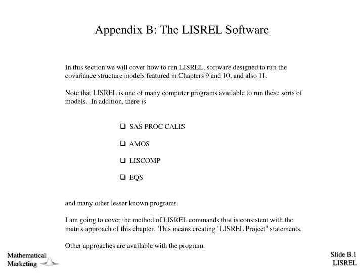
Appendix B: The LISREL Software. In this section we will cover how to run LISREL, software designed to run the covariance structure models featured in Chapters 9 and 10, and also 11.

Appendix B: The LISREL Software
E N D
Presentation Transcript
Appendix B: The LISREL Software • In this section we will cover how to run LISREL, software designed to run the covariance structure models featured in Chapters 9 and 10, and also 11. • Note that LISREL is one of many computer programs available to run these sorts of models. In addition, there is • SAS PROC CALIS • AMOS • LISCOMP • EQS and many other lesser known programs. I am going to cover the method of LISREL commands that is consistent with the matrix approach of this chapter. This means creating "LISREL Project" statements. Other approaches are available with the program.
Example from Johnson and Wichern p. 380 This example utilizes the difference in daily stock prices for five stocks picked from two industrial sectors. We hypothesize that the overall health of the two sectors is causally antecedent to the stock prices of the observed stock prices.
Chemicals Petroleum Allied Dupont Carbide Exxon Texaco Path Diagram of Johnson and Wichern Data
Example from Johnson and Wichern p. 380 DA NO=100 NI=5 LA Allied Dupont Carbide Exxon Texaco MO NY=5 NE=2 PS=SY,FR KM 1.000 .577 1.000 .509 .599 1.000 .387 .389 .436 1.000 .462 .322 .426 .523 1.000 FR LY(2,1) LY(3,1) LY(5,2) PS(2,1) MA LY 1 0 .4 0 .4 0 0 1 0 .4 MA PS 1 -.2 1 ST 1 TE(1) - TE(5) OU NS AL Title Statement Describes the DAta LAbels the variables Describes the MOdel Input Matrix FRee certain elements LISREL Program Statements Start values for y Start values for Start values for OUtput parameters
An Overview of Control Statements First statement is the title DAta parameters NO Number of observations NI Number of variables MA Matrix to be analyzed (= KM, CM, MM) xx n.nn n.nn n.nn n.nn n.nn n.nn … … … LA first-var-name second-var-name ···
The MOdel Parameters Statement MOdel parameters NY Number of Y variables NX Number of X variables NE Number of Eta variables NK Number of Ksi variables (All of these default to 0) ma can be any of the 8 LISREL parameter matrices: LY, TE, LX, TD, GA, BE, PH, PS FU SY DI ZE ID FI FR , ma =
Creating Start Values ST x.xx ma(m1, n1) ma(m2, n2) ••• Specify a particular value for various elements ma x x ··· x x x ··· x ··· ··· ··· ··· x x ··· x Specify a whole matrix filled with values ma can be LY, TE, LX, TD, GA, BE, PH or PS
Fixing or Freeing Indivual Elements • Priority Sequence: • Specification on a FI or FR statement • Specification in the MO statement • Default for that matrix FI ma(m1, n1) ma(m2, n2) ••• FR ma(m1, n1) ma(m2, n2) •••
The OUtput Parameters Statement OU TV MI NS
Special Cases y = y + x = x + = B + + V() = V() = V() = V() = • A confirmatory factor model with all y's • A confirmatory factor model with all x's • A structural equation model with all variables observed • A stuctural equation model with all y's