More on Stock Pollutants followed by the Environment and Asymmetric Information

1. More on Stock Pollutants followed by the Environment and Asymmetric Information Lecture ECON 4910

2. First some important OC results • Let V(x*,s)=max ∫s∞U(u,x)e-rtdt st dx/dt =f(x,u), x(s) = x* • The Hamiltonian is H = U(u,x) + f(x,u) • V(x*,s) has the following important properties: • dV/dx* = the co-state =  • dV/ds = -The Hamiltonian discounted = –U(u,x)e-rs – e-rsf(x,u) = the value of today’s consumption plus net investment.

3. An aggregate dynamic model • Representative consumer with utility function U(C,E). C is consumption and E is environmental pressure. (Alternatively a social welfare function) • E= E(S, F) where S is stock of pollutants and F is flow of pollutants. Positive derivatives. • Production is given by the production function Q(K,F). K is capital. Positive derivatives. • Production can be used for capital production and consumption. Q(K,F) = dK/dt + C, K(0) given • dS/dt = F – δS, S(0) given

4. The Economic Desicion Problem • max ∫∞U(C,E(S,F))e-rtdt • s.t: dS/dt = F – δS and dK/dt= Q(K,F) – C A problem with two state variables, K and S, and two control variables, C and F. First define the Hamiltonian: H= U(C,E(S,F)) + λ(Q(K,F) – C) + μ(F – δS)

5. Neccessary Conditions (kinda sorta) • C and F should maximize the Hamiltonian • (1) U’c – λ = 0 • (2) U’E E’F + λQ’F + μ = 0 • Differential equations for co-states (3) dμ/dt = rμ – U’EE’S + μδ (4) dλ/dt = rλ – λQ’K

6. Interpreting results • The model have some results from standard investment theory and some results from environmental theory

7. Results • U’c = λ marginal utility should equal marginal value of K. Differentiate and insert from (4) gives • dU’c/dt = λ(r – Q’K) If marginal productivity of capital is smaller than interest rate, then dU’c/dt is positive. This implies that C is a decreasing function of time. (You eat capital at diminishing rate.) In steady state, marginal productivity = discount rate

8. More results • From (2) λQ’F = – U’E E’F – μ. • The marginal value of F as input in production should equal the marginal disutility of F today + the cost of having one more unit of bad in the atmosphere. • May in steady state be written: • -U’E(E’F+E’S(r+δ)-1) = λQ’F • Left side is total marginal damage from F. Right side is value of marginal productivity of F.

9. How to implement the solution • Impose a dynamic tax τ • The firm wants to maximize p(t)Q(K,F) – rK – τF If there are no costs in transforming consumer wealth into capital then the price of capital is r = λ and will be taken care of by the market. Further in a market, price will be found by p(t)U’C = r p(t)Q’F = τ → optimal tax is τ = -r-1U’C(U’E E’F+μ).

10. NNP revisited • Return to the problem: Max ∫s∞U(C,E(S,F))e-rtdt s.t: dS/dt = F – δS and dK/dt= Q(K,F) – C • One can show that: • (dV/ds)s=0 = –U(C,E(S,F)) – (λ(Q(K,F) – C) + μ(F – δS)) Interpretation is that this is what we would loose if we where born at time s + 1. The welfare from living at time s = The Hamiltonian. Instantaneous welfare is then the Hamiltonian!

11. Hamiltonian and NNP • NNP is market value of consumption and investment. PCC + PII. • Now write U(C,F) as U’CC + U’FF. Then the Hamiltonian is • U’CC + U’FF + (λ(Q(K,F) – C) + μ(F – δS)). If we have a working market where prices are correct, then one can write this as • PCC + PFF + PII + change in pollution • If we use NNP PCC + PII then the NNP is not a measure of welfare. If it is working and prices are optimal, the NNP is a measure of welfare.

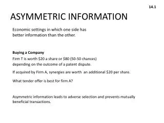
12. Environmental regulation with asymmetric information • Look at a firm with that produces a one unit of a good with profits. If the firm is unregulated the firm pollutes z. It can reduce the pollution by an amount z – x where x is actual level of pollution. The firm is taxed an amount T. • U = π – T – θ(z-x) is the firms profit. • The taxpayers has an utility function V=T – D(x), D’(x) > 0 and D’’(x) > 0 • The Government has an utility function W=V + αU 0 ≤ α < 1. Note definition of variables Thanks to Jon Vislie for coming up with a suitable model.

13. Features of model • A model of adverse selection • If type was known, D’(xi) = θi would define optimal solution for both types.

14. Source of asymmetry • The parameter θ may be θH or θL with θH > θL. The true value of θ is unknown to the government. • The government tries to give the firms a set of contracts. These contracts consists of a tax and a emission level. The firm wants to offer contracts such that the H firm takes the H contract and the L firm take the L contract. • Contract intended for H firm is {TH, xH}. Contract intended for L firm is {TL, xL}

15. Contracts • Participation constraints • (1) UL = π – TL – θL(z – xL) ≥ 0 • (2) UH = π – TH – θH(z – xH) ≥ 0 • Incentive constraints • (3) UL ≥ π – TH – θL(z – xH) • (4) UH ≥ π – TL – θH(z – xL) • One can show that there is no point in giving the H firm more than zero profit and that the L firm must be given a bonus for telling the truth. This implies that (2) and (3) are binding whereas (1) and (4) is not.

16. Showing that (1) and (4) are not binding • First one can try to calculate values of {TH, xH} and {TL, xL} under the assumption that all constraints are binding. That will not work neither will attempts with 3 binding constraints. • The reason? The set of equations is not linearly independent. Try solving the problem with matrix algebra and you will get a determinant equal to zero.

17. So let us try with (2) and(3) binding. • Implies (5) π – TH – θH(z – xH) = 0 (6) π – TL – θL(z – xL) = π – TH – θL(z – xH) From (6) calculate that: TL + θL(z – xL) – θL(z – xH) = TH Insert for TH into (5) gives (7) TL = π – θL(z – xL) –(θH – θL)(z – xH). Finally, inserting this expression for TL into (1) gives (8) UL = (θH – θL)(z – xH) ≥ 0 (>0 if xH < z.) This proves that (1) is not binding in the economic sense as it will hold automatically. Similar argument can be used to show that (4) is not binding unless it turns out that the high cost firm must abate more than the low cost firm. This is unlikely, but should formally be checked. (Insert UH = 0 and TL from 7 into (4) should do the trick)

18. The binding constraints are: • π – TH – θH(z – xH) = 0 • π – TL – θL(z – xL) = π – TH – θL(z – xH) • Participation for the high cost firm • Incentive compatibility for low cost firm • Let p be the probability of the firm being L • The regulator the solves the problem of maximizing E(W) subject to the above constraints • E(W) = p(TL – D(xL) + α(π – TL – θL(z – xL))) + (1 – p)(TH – D(xH) + α(π – TH – θH(z – xH)))

19. Solving the problem • Two possible approaches. In class we did direct insertion after solving constraints for of TL and TL. Her we use Lagrange methods. • Define Lagrangian: Λ = p(TL – D(xL) + α(π – TL – θL(z – xL))) + (1 – p)(TH – D(xH) + α(π – TH – θH(z – xH))) – λ(π – TH – θH(z – xH)) – μ(π – TL – θL(z – xL) – π + TH + θL(z – xH))

20. First order conditions • In addition to the constraints we get: (9) ∂Λ/∂TL = p – pα + μ = 0 (10) ∂Λ/∂TH = (1 – p) – (1 – p)α + λ – μ = 0 (11) ∂Λ/∂xL = –pD’(xL) + pαθL – μθL = 0 (12) ∂Λ/∂xH = –(1 – p)D’(xH) + (1 – p)αθH – λθH – μθL = 0

21. Results • From (9), μ = –(1 – α)p • Inserting μ = –(1 – α)p into (1) gives λ = α – 1. • Inserting μ = –(1 – α)p into (11) gives: D’(xL) = θL. Important result. If the firm is low cost firm it should be given a contract so that it behaves like first best. ”No distortion on the top”.

22. More results • Inserting from (9) and (10) into (12) and rearrange a bit gives the following expression: (1 – p)-1{θH(1 – αp) – (1 – α)pθL} = D’(xL) • Is xH larger/smaller than first best defined by D’(x*) = θH? • Remember that -D’’(xH) < 0. • If D’(xH) > θH then D’(xH) > D’(x*) which implies xH > x* because of the the convexity of D().

23. Graphical illustration. Higher D’(x) implies higher x. D(x) θ(z-x) x*

24. So. Is xH higher than x*? • If so, then: (1 – p)-1{θH(1 – αp) – (1 – α)pθL} > θH. This expression may be rewritten θH ≥ θL As which is true by assumption so xH is in fact higher than x*.

25. A loose thread • From slide 17. ” Similar argument can be used to show that (4) is not binding unless it turns out that the high cost firm must abate more than the low cost firm. This is unlikely, but should formally be checked. ” • We have that D’(xL) = θL and that D’(xH) > θH > θL. This implies that xH > xL. • Formal check concluded.

26. Summing up • Optimal contracts ensure that: • The low cost firm is efficient and makes a profit. • The high cost firm pollutes too much relative to first best and makes no profit. • Interesting dichotomy between efficiency in the real economy and efficiency in transfer economy