Download
1 / 54
540 likes | 656 Vues
This paper addresses the challenges of coordinating real-time autonomous agents in networked environments where tasks from multiple sources may conflict. It explores the importance of identifying critical conditions requiring coordination to optimize task execution without excessive negotiation. The proposed solutions include hierarchical plan representations and summary information to guide conflict resolution and enhance operational efficiency. An experimental domain involving transport agents and evacuee routing illustrates the effectiveness of these methods. The findings aim to improve coordination mechanisms and reduce unnecessary actions in dynamic settings.

E N D
Multilevel Coordination Mechanisms for Real-Time Autonomous Agents Edmund H. Durfee (PI) Brad Clement and Pradeep Pappachan (RAs) University of Michigan Update: February 2000
The Problem • Networked execution infrastructure permits concurrent, asynchronous initiation of tasks • Tasks originating from different sources might impose conflicting conditions on resources, services, and states of the world • Exactly which conditions matter might be decided during execution, and change dynamically • Identifying which (often few) conditions require coordination (typically negotiation), when, and in what (temporal) combinations is non-trivial • Negotiating over everything “just in case” can be wasteful, possibly myopic, and pose scaling difficulties
A Coalition Example • Joint Mission/Exercise with objectives/responsibilities distributed among multiple commands with their own human and computational agents • Operational choices within a command can unintentionally (infrequently) affect what others should or even can ultimately do (e.g., friendly fire) • “Grid” services should ensure that these interactions are efficiently predicted and effectively resolved • Resulting joint plan should: • Preserve room for some local run-time improvisation • Support efficient (fast, parallel) execution • Avoid unnecessarily costly actions • Require realistic runtime messaging load
Main Solution Ideas • Conditions to meet (on resource assignments, environmental parameters, etc.) are typically associated with plans that pursue tasks • Plans can be represented hierarchically, where abstract levels summarize the (alternative) activities they encompass • Abstract plans can be used to more efficiently discover potential conflicts (or lack thereof), and to guide search for details on conflicts • Choosing the right level for finding and resolving conflicts can balance coordination effort with the quality of concurrent activity and the robustness of plans.
crisper coordination lower cost coordination levels more flexibility Tradeoffs
Top-Down Search • Know as little as you can about others. • Use abstract resolutions to obviate deeper ones. • Reasoning at abstract levels is supported by “summary • information” from the deeper “and/or” plan tree blocked temporalconstraints
Summary Information Approach • Agents individually summarize what can or must happen in a plan subtree • Compare summary information to determine no coordination needed, to find coordinating commitments, or to guide deeper search • Coordinate prior to execution
Exploiting Summary Information • Prune inconsistent global plans (MightSomeWay) • “Expand most threats first” (EMTF) • expand subplan involved in most threats • focuses search on driving down to source of conflict • “Fewest threats first” (FTF) • search plan states with fewest threats first • or subplans involved in most threats are blocked first • Branch & bound - abstract solutions help prune space where cost is higher
Experimental Domain • Transports must carry evacuees to safe locations • Single lane routes • Routes may be destroyed • 4-12 locations • 2-4 transport agents
Summary Information vs. FAF FAF only returned with solutions to 6 of the 21 problems.
Summary Information vs. ExCon Points plotted where FTF-EMTF found optimal solution or both found a solution of same cost. FTF-EMTF found solutions for 16 out of 21 problems; DFS-ExCon found solutions for 8 out of 21.
Coordinating at higher levels is easier • This is not clear since summary information can grow exponentially up the hierarchy in the worst case. • Worst case complexity of deriving summary information is O(n2c2) for n plans in hierarchy each with O(c) conditions. • Checking the consistency of an ordering of n abstract plans each with O(c) summary conditions is O(n2c2). • Independent of the level of abstraction, checking an ordering is O(b2dc2) for O(b) subplans for each plan with O(c) conditions and hierarchy depth d. • Finding a consistent synchronization of actions is equivalent to resolving threats, which is shown to be NP-complete with the number of plans. • The number of abstract plans grows exponentially down the hierarchy, so difficulty grows exponentially.
Temporal Constraint Modeling • Create a temporal constraint network of primitive operators (across agents). Edges labeled with temporal relation vectors from inter-operator analysis. • Incrementally augment network via top-down plan elaboration and resolve potential conflicts
Runtime Coordination Cycle • Receive reduction of some operator P. Add operators in the • reduction to the network. • To resolve a previously imposed constraint P, Q, T do: • Fix temporal relations between Q and the operators in the • reduction of P. Check consistency of temporal network. • Synchronize/Select operators when necessary, request new • reductions (new constraints) and block those operators. • Delete P, Q, T. Unblock P and Q if they are not involved • in any other unresolved constraints. • Repeat steps until there are no more unresolved constraints.
Coordination Example (Fine Grained Coordination) COORDINATION TIME 4-3 7-4 3-2 2-6 6-8 8-6 6-2 2-3 3-4 4-7 B 1029 214 329 529 14 114 229 429 629 729 SIGNAL 929 2-6 6-5 5-1 1-2 A 730 850 1070 970 241 341 WAIT TIME B Overlaps A (Link (3, 6) is broken)
Evaluating Multiagent Plans • Intelligent Coordination Algorithms must be able to evaluate candidate multiagent plans based on well defined performance metrics in order to select plans with high “quality”. • Metrics for plan evaluation should be: • Computationally tractable • Good predictors of plan quality • Able to capture important tradeoffs that agents might wish to make during plan execution • We selected the following metrics for plan evaluation: Plan Cost, Plan Reliability and Plan Reward.
A Coordination Problem (Evacuation Domain) 2 3 4 1 A 6 B 5 7 8
Plans for Transport Agents in the Evacuation Domain B A B-EVAC-8 A-EVAC-6-5 B47 B34 B74 B43 A12 A-LONG-EVAC B-SHORT-EVAC A-SHORT-EVAC B-LONG-EVAC B36 B68 B86 B63 A51 A26 A65 B26 B68 B32 B86 B23 B62 A21 A15 A51 A65 A56
Plan Cost • Plan Cost estimates the cost associated with primitive operator execution for a plan. • The cost of a plan operator in a hierarchical plan can be recursively computed as follows: • If the operator can be reduced uniquely to a sequence of lower level operators, its cost is the sum of the costs of those operators. • If the operator can be reduced in more than one way to sequences of lower level operators, its cost is defined as the average cost of each possible reduction.
Example • In the example, assume that the cost of traversing an edge is $100 and the cost of destroying an edge after traversing it is $200 . • Cost(A-SHORT-EVAC) = Cost(A26) + Cost(A65) + Cost(A51) = 200 + 100 + 200 = 500 • Cost(A-LONG-EVAC) = Cost(A21) + Cost(A15) + Cost(A56) + Cost(A65) + Cost(A51) = 100 + 100 + 100 + 100 + 200 = 600 • Cost(A-EVAC-6-5) = (Cost(A-SHORT-EVAC) + Cost(A-LONG-EVAC))/2 = (500 + 600)/2 = 550
Plan Reliability • Plan Reliability estimates the likelihood of a plan being executed successfully in a dynamic environment. • Reliability is a concern if a plan operator can be reduced in more than one way to achieve a subgoal depending on the conditions that exist at runtime and one of the reductions has to be selected a priorifor coordination purposes. • The Reliability Quotient (RQ) of an operator reduction is computed by the number of world states that it is equipped to handle relative to the sum total of all the states that alternative reductions can handle. The greater this ratio, the greater the reliability of the reduction, assuming that any world state is equally likely to occur. • Joint plans which have operators with higher reliability quotients are valued higher w.r.t. this criterion.
Example • In the example, the operator B-EVAC-8 is multiply-reducible; it can be reduced to either B-SHORT-EVAC or B-LONG-EVAC depending on the conditions at runtime. If edge (3,6) is usable, the agent will prefer the reduction B-SHORT-EVAC, otherwise it will apply the reduction B-LONG-EVAC. • Since reduction B-SHORT-EVAC is applicable only when (3,6) is usable and reduction B-LONG-EVAC is preferred only if (3,6) is unusable, both reductions are mutually exclusive w.r.t. their applicability. • Suppose the number of states in which in which either reduction is applicable is n. With no prior knowledge of the probability that (3,6) will be usable in the future, the number of states in which either reduction will be applicable is assumed to be n/2. • Hence RQ(B-SHORT-EVAC) = RQ(B-LONG-EVAC) = (n/2)/n = 0.5
Plan Reward • Agents get rewards for successfully completing their plans. Rewards are assumed to be a function of plan execution time. Smaller times correspond to greater rewards and greater times to smaller rewards. • Plan reward estimates the reward that a joint plan is likely to yield. • Plan reward is computed by estimating the completion times for various agent plans under the constraints of a joint plan and calculating the rewards with the help of a pre-defined reward function. • Multiagent plans with higher levels of concurrency are rewarded more than those with less concurrency.
A26 B-EVAC-8 A26 B-EVAC-8 During(A26, B-EVAC-8) After(A26, B-EVAC-8) (a) (b) Example • Two different orderings of operators (from different candidate joint plans) is shown. Assume that it takes 200 min to traverse an edge. • The average completion times for A26 and B-EVAC-8 are 600 and 1000 resp. in (a) and 1000 and 1200 resp. in (b). • Reward function is defined as the negative of the maximum of the completion times of the individual plans. • Reward for joint plan in (a) = -max(600,1000) = -1000 Reward for joint plan in (b) = -max(1000, 1200) = -1200 Therefore, (a) is preferred to (b) under this criterion.
Selecting Multiagent Plans based on Tradeoffs • Agents might wish to make tradeoffs while selecting a joint plan for execution. • Examples of possible tradeoffs are: greater reward for lesser reliability, greater reliability for greater plan cost etc. • The multiagent plan evaluation algorithm must be able to evaluate candidate plans based on the tradeoffs that agents wish to make. • We adopt a technique used to solve multi-criteria decision problems to evaluate candidate multiagent plans based on agent tradeoffs.
Using Multi-criteria Decision Problem Solving Techniques for Evaluating Candidate Plans • In MCDPs it is necessary to evaluate available alternatives w.r.t. several criteria. • To solve such problems it is necessary to compute the value of the alternatives w.r.t. each criteria and also ascertain the relative importance of the criteria (tradeoffs). • The Ratio-scale method that we use, takes as input a matrix (ratio-scale matrix) that captures the relative importance of the criteria. This matrix is used to derive weights corresponding to each criterion. The value of an alternative (candidate joint plan) is the sum of its values w.r.t. each criterion weighted by the weight derived for that criterion from the ratio-scale matrix.
Plan Evaluation Algorithm • For each candidate joint plan, compute the Cost, Reliability and Reward measures. • From these measures compute the preference score for each candidate w.r.t. each criterion. The preference score of a candidate w.r.t. a criterion is the number of candidates with lower measures w.r.t. that criterion. • Using the weights (for the criteria) derived from the Ratio-scale matrix, compute the weighted sum of the preference scores for each candidate. • Select the candidate joint plan with the highest weighted sum, breaking ties arbitrarily.
Experiments (contd.) • Evacuation domain with three agents. Agents A and B have to evacuate from node 7 and C has to evacuate from 9. All routes are non-shareable and each agent has several routes. Edge (4,9) is the only edge that can fail with probability p. The cost and time for traversing edges is the same except for edge (6,7) which has a higher cost. • Number of different solutions possible with different tradeoffs between plan cost, reward and reliability. The graph compares three strategies S1, S2 and S3 for different values of p. The y axis represents normalized net reward (total reward - total cost for all the agents combined). The values have been normalized w.r.t. the value computed by the oracle which is assigned a uniform maximum reward of 1. • S1 corresponds to Reliability > Reward > Cost, S2 corresponds to Reward > Reliability > Cost, and S3 is a random strategy.
Experimental Results • At low values of p, S2 dominates S1 because the reliability measure which is heavily weighted in S1 conservatively assumes that the likelihood of edge (4,9) failing is 0.5. • At higher values of p, S1 dominates the other strategies and it finds the most reliable solution and it performance matches the oracle when p = 1. • S2 finds the most efficient (concurrent) solution and its performance matches the oracle when p = 0. • S1 consistently outperforms the random strategy S3 except at very low values of p.
Limitations of the Algorithm • The Reward measure adopts a greedy approach while computing the extent of concurrency between various plans in a joint plan by looking only at a subset of plans involved in constraints being resolved at the current stage of the hierarchical coordination process. When there are several plans in a joint plan space, the temporal orderings of a subset of plans might very well affect the completion times of plans outside that subset. • The algorithm is sensitive to the preference intensities assigned to the various criteria. E.g., observed that if the preference for reliability over reward in S1 was below a threshold, the reward and cost criteria combined dominated the reliability criterion, yielding less reliable solutions. • The order in which the coordination process resolves various conflicts and the individual preferences of the agents for certain plans also impacts the quality of the solutions.
Factory Domain Agents and their Tasks • There are three agents: • Production Manager: Processes raw parts to produce new products. • Inventory Manager: Makes parts available for processing and stows finished products. • Facilities Manager: Services machines. • Constraints: • Raw parts and finished products occupy pre-designated slots. • Only one part or finished product can occupy a slot at a time. Therefore parts or finished products must be stowed in the warehouse to make room for new ones. • Some machines must be freed for servicing some time during the day.
Factory Domain PRODUCTION MANAGER PARTS ON FACTORY FLOOR M2 M1 M3 C D A B B A/AB/E C/CD/F D FACILITIES MANAGER INVENTORY MANAGER RAW PARTS T1 E F T2 FINISHED PRODUCTS T3 AB CD TOOL AREA WAREHOUSE
Plan for the Production Manager Production_Plan Make_AB Make_CD Process(M1,A,Ø,A’) Process(M2,A’,B,AB) Process(M2,C,Ø,C’) Process(M,P1,P2,OP) Pre: free(M) available(P1) available(P2) In : ~free(M) ~available(P1) ~available(P2) Out: free(M) available(OP) ~available(P1) ~available(P2) Process(M3,C’,D,CD) Process(M1,C’,D,CD)
Plan for the Inventory Manager Inventory_Plan Open(E) Open(F) Pickup(E) Swap(E,A) Swap(E,AB) Pickup(F) Swap(F,C) Swap(F,CD) Pickup(P) Pre: ondock(P) In: ~ondock(P) Post: available(P) Stow(P) Pre: available(P) In: ~available(P) available(P) Post: ~available(P) Swap(P1,P2) Stow(P1) & Pickup(P2)
Plan for the Facilities Manager Service_Plan Service_M2 Service_M1 Service_M3 Equip(M1,T1) Maintain(M1) Equip(M2,T2) Maintain(M2) Equip(M3,T3) Maintain(M3) Equip(M, T) Pre: ~holding(T) free(M) In : holding(T) free(M) ~free(M) Out: holding(T) free(M) Maintain(M, T) Pre: holding(M,T) free(M) In : ~free(M) free(M) holding(M,T) Out: free(M) holding(M,T)
Time = 42050.01 cpu sec. Time = 44014.65 cpu sec. Time = 5401.74 cpu sec. Trading Computation for Quality M1 - A’ M2 - AB M2 - C’ M3 - CD Swap E, AB Swap F, CD Service M1 Service M2 Service M3 M1 - A’ M2 - AB M2 - C’ M3 - CD Swap E, AB Swap F, CD Service M1 Service M3 Service M2 M1 - A’ M2 - AB M2 - C’ M3 - CD Swap E, AB Swap F, CD Service M3 Service M1 Service M2
Making Things More Concrete… • Need experimental domain(s) and system(s) to map qualitative characteristics into parameters and metrics • Realistic domain • Easier to justify; must address aspects like-it-or-not • Generalization can be challenging; limited experimental range; knowledge-engineering effort; harder to explain • Abstract domain • Lower entry cost; scale-up easier; versatility; sharability, explainability • Harder to motivate; “doomed to succeed”
Current Status • Algorithms have been implemented as Grid Ready Components • Experimentation on NEO and Factory domains to explore versatility/effectiveness • Analytical and experimental testing of cost and effectiveness of the algorithms, especially relative to other coordination/planning search techniques • Emerging techniques for evaluating alternative coordinated plans • Transitioning evaluation criteria into search heuristics
Abstract NEO Testbed Control/Brokering Techniques Java Implementation DM DM CORBA DM DM Computer/communication network
Concurrent Hierarchical Planner • HTN planning with concurrency and ability to reason at abstract levels • Soundness and completeness based on formalization of summary information • Exploiting summary information in search • Experimentally compare to others (Tsuneto et. al. ‘97) • Characterize plans where these heuristics better/worse
Summary Information pre: at(A,1,3)in: at(A,1,3), at(B,1,3), at(B,0,3), at(A,0,3), at(B,0,4), at(A,1,3) post: at(A,1,3), at(B,1,3),at(B,0,3), at(A,0,4), at(A,0,3),at(B,0,3), at(B,0,4) 1,3->0,4HI • must, may • always, sometimes • first, last • external preconditions • external postconditions 1,3->0,3 0,3->0,4 pre: at(A,1,3)in: at(A,1,3), at(B,1,3), at(B,0,3)post: at(A,0,3), at(A,1,3), at(B,1,3), at(B,0,3) pre: at(A,0,3)in: at(A,0,3), at(B,0,3), at(B,0,4)post: at(A,0,4), at(A,0,3), at(B,0,3), at(B,0,4) pre: at(A,1,3)in: at(A,1,3), at(B,1,3), at(B,0,3), at(B,1,4), at(A,0,3), at(A,1,4), at(B,0,4), at(A,1,3)post: at(A,1,3), at(B,1,3),at(B,0,3), at(A,0,4), at(A,0,3), at(A,1,4), at(B,0,3),at(B,1,4), at(B,0,4) 0 1 2 3 4 1,3->0,4 DA 0 A 1,3->0,4HI 1,3->0,4LO 1 DB 2 B
DA A DB B Determining Temporal Relations • CanAnyWay(relation, psum, qsum) - relationcan hold for any wayp and q can be executed • MightSomeWay(relation, psum, qsum) - relationmight hold for some wayp and q can be executed • CAW used to identify solutions • MSW used to identify failure • CAW and MSW improve search • CAW and MSW must look deeper • MSW identifies threats to resolve CanAnyWay(before, psum, qsum) ØCanAnyWay(overlaps, psum, qsum) MightSomeWay(overlaps, psum, qsum) B - before O - overlaps
Evaluating Multiagent Plans • Intelligent Coordination Algorithms must be able to evaluate candidate multiagent plans based on well defined performance metrics in order to select plans with high “quality”. • Metrics for plan evaluation should be: • Computationally tractable • Good predictors of plan quality • Able to capture important tradeoffs that agents might wish to make during plan execution • We selected the following metrics for plan evaluation: Plan Cost, Plan Reliability and Plan Reward.
Plan Cost • Plan Cost estimates the cost associated with primitive operator execution for a plan. • The cost of a plan operator in a hierarchical plan can be recursively computed as follows: • If the operator can be reduced uniquely to a sequence of lower level operators, its cost is the sum of the costs of those operators. • If the operator can be reduced in more than one way to sequences of lower level operators, its cost is defined as the average cost of each possible reduction.