Download
1 / 70
700 likes | 716 Vues
Part 3: discriminative methods. Discriminative methods. Object detection and recognition is formulated as a classification problem. The image is partitioned into a set of overlapping windows, and a decision is taken at each window about if it contains a target object or not.

E N D
Discriminative methods • Object detection and recognition is formulated as a classification problem. The image is partitioned into a set of overlapping windows, and a decision is taken at each window about if it contains a target object or not. • Each window is represented by extracting a large number of features that encode information such as boundaries, textures, color, spatial structure. • The classification function, that maps an image window into a binary decision, is learnt using methods such as SVMs, boosting or neural networks.
Overview • General introduction, formulation of the problem in this framework and some history. • Explore demo + related theory • Current challenges and future trends
Background Computer screen Bag of image patches In some feature space Discriminative methods Object detection and recognition is formulated as a classification problem. The image is partitioned into a set of overlapping windows … and a decision is taken at each window about if it contains a target object or not. Decision boundary Where are the screens?
Classification function Where belongs to some family of functions Formulation • Formulation: binary classification … x1 x2 x3 … xN xN+1 xN+2 xN+M … Features x = -1 +1 -1 -1 ? ? ? y = Labels Training data: each image patch is labeled as containing the object or background Test data
Formulation • The loss function • Find that minimizes the loss on the training
0.1 0.05 0 0 10 20 30 40 50 60 70 1 0.5 0 0 10 20 30 40 50 60 70 1 -1 0 10 20 30 40 50 60 70 80 Discriminative vs. generative • Generative model x = data • Discriminative model x = data • Classification function x = data
Classifiers • NN • SVM • K-NN, nearest neighbors • Additive models
Nearest neighbor classifiers Learning involves adjusting the parameters that define the distance
Object models • Invariance: search strategy • Part based • Template matching
Object models Big emphasis on the past on face detection: It provided a clear problem with a well defined visual category and many applications. It allowed making progress on efficient techniques. • Rowley • Scheiderman • Poggio • Viola • Ullman • Geman
A simple object detector with Boosting • Download • Toolbox for manipulating dataset • Code and dataset • Matlab code • Gentle boosting • Object detector using a part based model • Dataset with cars and computer monitors http://people.csail.mit.edu/torralba/iccv2005/
Boosting • A simple algorithm for learning robust classifiers (Shapiro, Friedman) • Provides efficient algorithm for sparse visual feature selection (Tieu & Viola, Viola & Jones)
Boosting • Defines a classifier using an additive model: • We need to define a family of weak classifiers Strong classifier Weak classifier Weight Features vector from a family of weak classifiers
+1 ( ) yt = -1 ( ) Boosting • It is a greedy procedure: xt=1 Each data point has a class label: xt xt=2 and a weight: wt =1
+1 ( ) yt = -1 ( ) Toy example Weak learners from the family of lines Each data point has a class label: and a weight: wt =1 h => p(error) = 0.5 it is at chance
+1 ( ) yt = -1 ( ) Toy example Each data point has a class label: and a weight: wt =1 This one seems to be the best This is a ‘weak classifier’: It performs slightly better than chance.
+1 ( ) yt = -1 ( ) Toy example Each data point has a class label: We update the weights: wt wt exp{-yt Ht} We set a new problem for which the previous weak classifier performs at chance again
+1 ( ) yt = -1 ( ) Toy example Each data point has a class label: We update the weights: wt wt exp{-yt Ht} We set a new problem for which the previous weak classifier performs at chance again
+1 ( ) yt = -1 ( ) Toy example Each data point has a class label: We update the weights: wt wt exp{-yt Ht} We set a new problem for which the previous weak classifier performs at chance again
+1 ( ) yt = -1 ( ) Toy example Each data point has a class label: We update the weights: wt wt exp{-yt Ht} We set a new problem for which the previous weak classifier performs at chance again
Toy example f1 f2 f4 f3 The strong (non- linear) classifier is built as the combination of all the weak (linear) classifiers.
Boosting • Different cost functions and minimization algorithms result is various flavors of Boosting • In this demo, I will use gentleBoosting: it is simple to implement and numerically stable.
gentleBoosting GentleBoosting fits the additive model by minimizing the exponential loss Training samples Minimization is perform Newton steps
gentleBoosting Iterative procedure. At each step we add We chose that we minimizes the cost: A Taylor approximation of this term gives: At each iterations we just need to solve a weighted least squares problem Weights at this iteration For more details: Friedman, Hastie, Tibshirani. “Additive Logistic Regression: a Statistical View of Boosting” (1998)
Weak classifiers • Generic form • Regression stumps: simple but commonly used in object detection. • Decision tree fm(x) b=Ew(y [x> q]) a=Ew(y [x< q]) Four parameters: x q
gentleBoosting.m function classifier = gentleBoost(x, y, Nrounds) … for m = 1:Nrounds fm = selectBestWeakClassifier(x, y, w); w = w .* exp(- y .* fm); % store parameters of fm in classifier … end Initialize weights w = 1 Solve weighted least-squares Re-weight training samples
Demo gentleBoosting Demo using Gentle boost and stumps with hand selected 2D data: > demoGentleBoost.m
Probabilistic interpretation • Generative model • Discriminative (Boosting) model It can be a set of arbitrary functions This provides a great flexibility, difficult to beat by current generative models. But also there is the danger of not understanding what are they really doing.
From images to features:Weak detectors We will now define a family of visual features that can be used as weak classifiers (“weak detectors”)
Weak detectors Textures of textures Tieu and Viola, CVPR 2000 Every combination of three filters generates a different feature This gives thousands of features. Boosting selects a sparse subset, so computations on test time are very efficient. Boosting is also very robust to overfitting.
Weak detectors Haar filters and integral image
Weak detectors Edge probes & chamfer distances
Weak detectors Part based: similar to part-based generative models. We create weak detectors by using parts and voting for the object center location Screen model Car model These features are the ones used for the detector on the course web site.
Weak detectors We can create a family of “weak detectors” by collecting a set of filtered templates from a set of training objects. * = = Better than chance
Weak detectors We can do a better job using filtered images Still a weak detector but better than before We can create a family of “weak detectors” by collecting a set of filtered templates from a set of training objects.
From images to features:Weak detectors First we create a family of weak detectors. 1) We collect a set of filtered templates from a set of training objects. 2) Each weak detector works by doing template matching using one of the templates.
Weak detectors • Generative model • Discriminative (Boosting) model Image fi, Pi Feature gi Part template Relative position wrt object center
Training First we evaluate all the N features on all the training images. Then, we sample the feature outputs on the object center and at random locations in the background:
Example of weak ‘screen detector’ We run boosting: At each iteration we select the best feature on the weighted classification problem: hm (v) A decision stump is a threshold on a single feature Each decision stump has 4 parameters: {f, q, a, b} f = template index (selected among a dictionary of templates) q = Threshold, a,b = average class value (-1, +1) at each side of the threshold
… … 1 2 3 4 10 100 Representation Selected features for the screen detector
Representation Selected features for the car detector … … 100 3 2 4 1 10
Example: screen detection Feature output
Example: screen detection Thresholded output Feature output Weak ‘detector’ Produces many false alarms.
Example: screen detection Thresholded output Feature output Strong classifier at iteration 1
Example: screen detection Thresholded output Feature output Strong classifier Second weak ‘detector’ Produces a different set of false alarms.
Example: screen detection Thresholded output Feature output Strong classifier + Strong classifier at iteration 2
Example: screen detection Thresholded output Feature output Strong classifier + … Strong classifier at iteration 10
Example: screen detection Thresholded output Feature output Strong classifier + … Adding features Final classification Strong classifier at iteration 200
Demo Demo of screen and car detectors using parts, Gentle boost, and stumps: > runDetector.m