Download
1 / 26
260 likes | 414 Vues
Rick Lumpkin (Rick.Lumpkin@noaa.gov) National Oceanic and Atmospheric Administration (NOAA) Atlantic Oceanographic and Meteorological Laboratory (AOML) Miami, Florida USA Silvia Garzoli and Gustavo Goni NOAA/AOML Peter Niiler NOAA/JIMO. GOOS/GCOS measurements of near-surface currents.

E N D
Rick Lumpkin (Rick.Lumpkin@noaa.gov) National Oceanic and Atmospheric Administration (NOAA) Atlantic Oceanographic and Meteorological Laboratory (AOML) Miami, Florida USA Silvia Garzoli and Gustavo Goni NOAA/AOML Peter Niiler NOAA/JIMO GOOS/GCOS measurements of near-surface currents Office of Climate Observations 6th Annual System Review, 3 September 2008
Drifters + altimetry in the South Atlantic Brazil-Malvinas Confluence Shading: SSTA trend, 1993—2002 (C) from NCEP/NCAR.v2 reanalysis. Lumpkin & Garzoli (2008)
Latitude of the Brazil-Malvinas Confluence Trend: 0.860.06 degrees per decade Lumpkin & Garzoli (2008)
Latitude of maximum wind stress curl -1.060.56 degrees per decade Basin-averaged SST anomaly (°C) Lumpkin & Garzoli (2008)
Analogy with SST analysis:Potential Satellite Bias Error Satellite measurements Model Field at surface Biases in model: biases in resulting field. In-situ observations: reduce bias. Resulting bias error is a function of observing system configuration and biases in various platforms.
Near-surface currents What model converts satellite measurements to near-surface currents? OSCAR: the most mature satellite-based surface current product. Web page offers comparisons with moored and drifting buoys in various regions. However, the OSCAR currents aren’t accompanied by formal error bars needed to asses bias.
Drifter motion: Five-day lowpass: filter tides, inertial oscillations, submesoscale. GOAL: forecast surface velocities (and drifter trajectories) with wind and altimetry products, including error bars. Assess Potential Satellite Bias Error.
Ekman: Ralph and Niiler (1999), Niiler (2001). Geostrophic mean from hydrographic climatology, variations addressed by averaging in 2° 5° bins. Mean angle 54° off the wind. For NCEP winds, best fit A=0.081 s-1/2.
Geostrophic: For many studies (e.g., Rio and Hernandez, 2003), • Left: Altimeter EKE minus drifter EKE (Fratantoni, 2001). • Several reasons that these can differ in general, even if Ekman and slip are perfectly removed: • centrifugal force, submesoscale motion, etc. • mismatch between spatial smoothing of altimetry, temporal smoothing of drifters, and energy spectra of motion.
Absolute sea level height (cm) (from Niiler, Maximenko & McWilliams, 2003) Drifter measurements G(x) Drifter mean (biased) Unbiased mean SLA geo.vel.anomaly Niiler et al., (2003):
Best fit: A=0.07 Wind speed Drag area ratio Niiler et al., (1995), Niiler and Paduan (1995): Holey-sock drifters: R=40. Slip is 1.8 cm/s in 10 m/s wind. Pazan and Niiler (2001): uundrogued=udrogued+(7.910-3)W.
Slip in high wind/wave state Niiler et al. (1995) measurements of slip were in W8 m/s. Slip may exceeds linear relationship at high wind/wave state. Niiler, Maximenko and McWilliams (2003): absolute sea height change, 40—60°S: 2.34m, all drifters; 1.98m, only drifters in W8 m/s; 1.55 m, hydrography referenced to floats (Gille, 2003). Discrepancies with models: problems with models or with data? Left: mean zonal drifter speed (AOML climatology) minus mean zonal speed of ECCO-GODAE 1° state estimation, 15yr mean (figure courtesy M. Mazloff, WHOI). Consistent offset in Southern Ocean.
How we can improve our understanding of drifter motion? • Use high resolution scatterometer-based wind product and include ocean currents when calculating wind stress. • Simultaneously project motion into geostrophic, wind-driven, and residual components. Solve in bins using Gauss-Markov estimation. (Lumpkin and Elipot, in preparation)
Wind and wind stress Winds: 6 h, 25 km resolution Variational Analysis Method (VAM) product (Atlas et al., 1996; Atlas et al., 2008) derived from SSM/I, AMSR-E, TMI, QuickSCAT, SeaWinds, and in-situ observations and ECMWF analysis. Stress: Smith (1988) algorithm as implemented in COARE 3.0 (Fairall et al., 2003) applied to VAM wind and drifter downwind speed (if drifter speed=wind speed, stress=0).
Results Globally-averaged gain: 1.13±0.06
Where do these results differ from RN99? a: using significant wave height. w: using peak wave period.
Summary Within assumed error, 5d lowpassed drifter velocities can be estimated as sum of geostrophic and wind-driven. Residual has structure related to EKE maxima. AVISO altimetry generally underestimates observed EKE, presumably due to smoothing in OI. But some regions are overestimated with a gain of 1. Ageostrophic terms in surface momentum budget. Wind-driven component is consistent with Ralph and Niiler (1999) in much of the tropics, subtropics. However, high wind areas have larger downwind motion. The spatial variations in the wind-driven part may be due to Stokes drift in wave field. This will be included explicitly in the next version of the model. Stokes drift: 10—20 cm/s increase in time-mean, in some regions of the Southern Ocean.