DNA sequence 분석방안
DNA sequence 분석방안. 인지과학협동과정 이수화 김준식 유전공학협동과정 김수동. Feed-forward backpropagation network. Network 구성 Exon 과 non-exon sequence 의 구별 Matlab 5.3 의 newff 함수 이용 {A, C, G, T} -> {1, 2, 3, 4} 로 변환 Window size = 30 Hidden layer node -> 25 개 , Output node -> 1 개


DNA sequence 분석방안
E N D
Presentation Transcript
DNA sequence 분석방안 인지과학협동과정 이수화 김준식 유전공학협동과정 김수동
Feed-forward backpropagation network • Network 구성 • Exon과 non-exon sequence의 구별 • Matlab 5.3의 newff 함수 이용 • {A, C, G, T} -> {1, 2, 3, 4}로 변환 • Window size = 30 • Hidden layer node -> 25개, • Output node -> 1개 • 269개 sequence로 training(exon & non-exon) • MSE로 training결과 분석
함수 상세 • net=newff([1 4; 1 4; 1 4; 1 4; 1 4; 1 4; 1 4; 1 4; 1 4; 1 4; 1 4; 1 4; 1 4; 1 4; 1 4; 1 4; 1 4; 1 4; 1 4; 1 4; 1 4; 1 4; 1 4; 1 4; 1 4; 1 4; 1 4; 1 4; 1 4; 1 4], [25,1],{'tansig','purelin'},'traingd') • ‘tansig’ : n = 2/(1+exp(-2*n))-1, ‘traingd’ = dX = lr * dperf/dX TRAINGD, Epoch 9775/10000, MSE 0.0110698/0, Gradient 0.0181744/1e-010 TRAINGD, Epoch 9800/10000, MSE 0.0109876/0, Gradient 0.0180941/1e-010 TRAINGD, Epoch 9825/10000, MSE 0.0109061/0, Gradient 0.0180142/1e-010 TRAINGD, Epoch 9850/10000, MSE 0.0108253/0, Gradient 0.0179346/1e-010 TRAINGD, Epoch 9875/10000, MSE 0.0107452/0, Gradient 0.0178553/1e-010 TRAINGD, Epoch 9900/10000, MSE 0.0106659/0, Gradient 0.0177764/1e-010 TRAINGD, Epoch 9925/10000, MSE 0.0105872/0, Gradient 0.0176979/1e-010 TRAINGD, Epoch 9950/10000, MSE 0.0105093/0, Gradient 0.0176198/1e-010 TRAINGD, Epoch 9975/10000, MSE 0.010432/0, Gradient 0.0175421/1e-010 TRAINGD, Epoch 10000/10000, MSE 0.0103554/0, Gradient 0.0174647/1e-010
Poor result에 대한 분석 • Exon-non exon간의 데이터 차별성이 있는가? • Node의 수 (window size, hidden nodes..) • Training Data의 크기 • 동일 종, 동일 단백질을 형성하는 DNA set.. • (e.g. Aplysia, 18S rRNA …)
HMM-EM Model* • Main states : 4 {A, C, G, T} • Observation States : 4 {A, C, G, T} • Matrix 구성 • Prior matrix = M x 1 = 4 x 1 • Transition matrix = M x M = 4 x 4 • Observation matrix = M x O = 4 x 4 • Prior, Transmat, Obsmat 각각의 최초 임의 값으로 할당 • Baum-Welch EM algorithm으로 matrix의 parameter 추정 * http://www.cs.berkeley.edu/~murphyk/Bayes/hmm.html
HMM-EM Model 2 [LL, PRIOR, TRANSMAT, OBSMAT] = LEARN_HMM(DATA, PRIOR0, TRANSMAT0, OBSMAT0) % computes maximum likelihood estimates of the following parameters, % where, for each time t, Q(t) is the hidden state, and % Y(t) is the observation % prior(i) = Pr(Q(1) = i) % transmat(i,j) = Pr(Q(t+1)=j | Q(t)=i) % obsmat(i,o) = Pr(Y(t)=o | Q(t)=i) % It uses PRIOR0 as the initial estimate of PRIOR, etc.
HMM-EM 상세* % initial guess of parameters, Q=4(main states), O=4 (observation) prior1 = normalise(rand(Q,1)); transmat1 = mk_stochastic(rand(Q,Q)); obsmat1 = mk_stochastic(rand(Q,O)); % improve guess of parameters using EM max_iter = 500; [LL, prior2, transmat2, obsmat2] = learn_dhmm(data, prior1, transmat1, obsmat1, max_iter); % use model to compute log likelihood loglik = log_lik_dhmm(data, prior2, transmat2, obsmat2)
결과 • 990개의 exon sequence로 training prior1 = 0.2912 0.1266 0.2098 0.3725 prior2 = 0.3365 0.1776 0.2067 0.2792 transmat1 = 0.0613 0.2321 0.3834 0.3232 0.1156 0.0446 0.4218 0.4180 0.5740 0.0134 0.1157 0.2968 0.1919 0.0783 0.4864 0.2434 transmat2 = 0.0450 0.3388 0.0441 0.5720 0.1371 0.0027 0.7965 0.0637 0.5104 0.0328 0.3451 0.1117 0.2575 0.0982 0.1458 0.4985 obsmat1 = 0.1295 0.4131 0.3147 0.1427 0.0466 0.0943 0.6805 0.1786 0.2989 0.0153 0.6762 0.0096 0.1679 0.3332 0.1412 0.3577 obsmat2 = 0.2010 0.4508 0.3094 0.0389 0.4911 0.0224 0.0080 0.4785 0.1196 0.0031 0.6836 0.1936 0.2813 0.4111 0.0059 0.3017
18S rRNA : 종간 유연관계 식별 • 모든 진핵생물에 고르게 분포 • 계통수 작성에 사용하는 지표 분자