Cellular Automaton Wave Propagation Models of Water Transport Phenomena in Hydrology Robert N. Eli

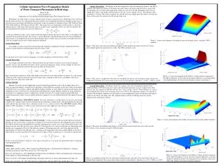
1. Cellular Automaton Wave Propagation Models of Water Transport Phenomena in Hydrology Robert N. Eli Associate Professor Department of Civil and Environmental Engineering, West Virginia University Hydrology is the study of the occurrence and movement of water in natural systems. Hydrologists have observed that the motion of water over and beneath the earth’s surface can be adequately described by the physical processes of advection (mass movement) and diffusion (attenuation) in the vast majority of situations (Ponce 1989, Wurbs & James 2002, Abbott & Basco 1989, Bear & Verruijt 1987). This means that wave propagation can be treated as a advection-diffusion process rather than a fully dynamic process (in other words, momentum effects can safely be ignored). The governing differential equation for advection-diffusion is: x is the space dimension and t is time, and h is either the depth of the flowing water on the surface, or the depth of the saturated soil in ground water flow. The velocity c and the diffusion coefficient D dictate the advection and diffusion characteristics of the property h in the particular hydrologic process (either surface water flow or ground water flow). i is the rate of depth increase due to either rainfall or infiltration. Surface Water Flow An example of surface water flow is that produced by rainfall on a parking lot. In this example the advective velocity c and the diffusion coefficient D are given by (Ponce 1989): S is the slope of the surface and n is Manning’s n (a surface roughness coefficient (Ponce 1989)). Ground Water Flow An example of ground water flow is that produced by the movement of water in a layer of porous granular material, such as sand, bounded on the lower side by a horizontal impervious surface. In this example the advective velocity c and the diffusion coefficient D is given by (Bear & Verruijt 1987): KH is the hydraulic conductivity of the sand (ability of the sand to let water flow without resistance), CS is the storage coefficient of the sand (fraction of the total sand volume that is available to hold water), and Δh/Δx is the rate of change of h in the x direction (slope of h). Solution Methods Equation [1] can be solved in application to practical hydrology problems (such as the examples above) by a range of numerical methods (computer-based algorithms). Finite difference methods are the most widely used and they are divided into two categories, explicit and implicit. Implicit methods are more difficult to program and require more computing resources in the form of calculation time and information storage. Explicit methods are easier to program and require less computing resources. Additionally, Cellular Automata (CA) and the explicit method (EM) share similar characteristics, hence a classic explicit method is compared to a new cell based method in this proof of concept study. Explicit Finite Difference (QUICKEST) method: The space dimension x is divided into a row of cells, each having a width of Δx, starting at time t. If the cell location in the x direction is indexed with j, then the depth h at the next time step t +Δt (the time increment is Δt) is a function of cells j-2, j-1, j, and j+1 at time t. The QUICKEST method (Abbott & Basco 1989) algorithm is 3rd order accurate (good accuracy) and is applied to each cell in the x direction: Conservative Mass Cellular Automata (CMCA) method: A serious concern with most finite difference methods is that they do not conserve mass, causing mass to appear to be created or destroyed as the computations proceed in time. The CMCA method avoids this problem by explicitly exchanging mass (in this case, water volume) between the cells during each time step. The advective water volume V [7] leaving each cell is sent to an adjacent cell, depending on the direction of uocomputed in [2] or [4]. The diffusive volume v [8] leaving each cell is sent to the adjacent cells by apportioning v to both the left and right cell as a function of the magnitude of the down gradient Δh/Δx to the left or right. If there is no down gradient in h to either the left or right, or both, no portion of v is sent to those adjacent cells. In [8], γ is given by [6] above, while CS= 1 for surface water flow, or is less than 1 for groundwater flow (see ground water paragraph above). References: Abbott, M.B. and Basco, D.R., 1989; Computational Fluid Dynamics, An Introduction for Engineers; Longman Scientific & Technical, John Wiley & Sons, Inc., New York, NY. Bear, A.V. and Verruijt, A., 1987; Modeling Groundwater Flow and Pollution, Theory and Applications of Transport in Porous Media; D. Reidel Publishing Co. Boston, MA. Ponce, Victor M., 1989; Engineering Hydrology, Principles and Practices; Prentice Hall, Englewood Cliffs, NJ. Wurbs, R.A. and James, W., 2002; Water Resources Engineering; Prentice Hall, Upper Saddle River, NJ. Surface Water Flow: The Figures in this box compare the results of running the Quickest and CMCA methods. The impervious surface is 200 meter long and 1 meter wide with a slope of 0.001 (1 m per 1000 m). Rainfall occurs over the entire length of the surface at a rate of 0.072 m/hr, beginning at time 0.0 and ending after 5 hours. The length is divided into 20 cells (Δx = 10 m), and Δt = 60 sec . The duration of the simulation is 10 hours. The surface is initially dry, and the water layer builds up on the surface over time and flows off the end of the surface at the 200 m end of the scale. Figure 3: A space-time diagram of the depth of water on the plane surface (using the CMCA method). Figure 1: This shows how the water builds up in depth over the length of the surface for the first 3 hours of the rainfall, plotted at equal intervals of time. The CMCA method is used. Figure 4: A space-time diagram of the diffusive volume transfer component of the CMCA simulation. It shows that the maximum diffusion is occurring during water depth buildup at the downstream boundary condition (a problem ?!) Figure 2: This shows a comparison of the flow rate (discharge) leaving the end of the plane surface for the two computational methods. The conservation of mass error for each method is: Quickest = -10.62% ; CMCA = 0.00% Ground Water Flow: The Figures in this box compare the results of running the Quickest and CMCA methods. A 200 meter long and 1 meter wide horizontal impervious surface is topped with a thick layer of sand. The length is divided into 20 cells (Δx = 10 m), and Δt = 300 sec . Water infiltrates at a rate of 0.036 m/hr into the sand in a zone extending from 45 m to 145 m. The infiltration continues for a period of 24 hours. The boundary conditions are equivalent to a vertical impervious barrier at 0 distance and exposed outflow at the 200 m end of the scale. The simulation begins with the sand being totally dry and the duration of the simulation is 60 days. Elapsed time, days Figure 3: A space-time diagram of the depth of saturated sand (using the CMCA method). Figure 5: This shows the buildup in the thickness of the saturated sand at equal intervals of time over the first 16 hours of the simulation using the CMCA method. Elapsed time, days Elapsed time, days Figure 4: A space-time diagram of the diffusive volume transfer component of the CMCA simulation. It shows that the maximum diffusion is occurring during the infiltration period at the beginning of the simulation, when water table slope changes are at their maximum (expected). Figure 6: A comparison of the flow rate (discharge) exiting from the sand at the 200 m end of the scale over the duration of the simulation. The conservation of mass error for each method is: Quickest = +6. 01% ; CMCA = +0.90%