Download
1 / 27
270 likes | 465 Vues
EarthCARE and snow. Robin Hogan, Chris Westbrook University of Reading Pavlos Kollias McGill University. 6 May 2013. Spaceborne radar, lidar and radiometers. EarthCare. EarthCARE (launch 2016) ESA+JAXA 400-km orbit: more sensitive 94-GHz Doppler radar

E N D
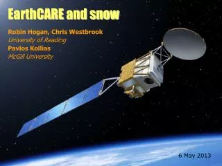
EarthCARE and snow Robin Hogan, Chris Westbrook University of Reading PavlosKollias McGill University 6 May 2013
Spaceborne radar, lidar and radiometers EarthCare • EarthCARE (launch 2016) • ESA+JAXA • 400-km orbit: more sensitive • 94-GHz Doppler radar • 355-nm HSRL/depol. lidar • Multispectral imager • Broad-band radiometer • Heart-warming name The A-Train (fully launched 2006) • NASA • 700-km orbit • CloudSat 94-GHz radar • Calipso 532/1064-nm depol. lidar • MODIS multi-wavelength radiometer • CERES broad-band radiometer • AMSR-E microwave radiometer
Overview • Introduction to unified retrieval algorithm (in development!) • What will EarthCARE data look like? • Quantification and correction of Doppler errors • What are the issues in extending algorithm to riming/unriming snow? • What’s the difference between ice cloud and snow? • How do we validate particle scattering models using real data? • Can we exploit EarthCARE’s Doppler to retrieve riming snow? • Your advice would be much appreciated! • Preliminary simulation of a retrieval of riming snow • Outlook
Unified retrieval Ingredients developed Not yet developed 1. Define state variables to be retrieved Use classification to specify variables describing each species at each gate Ice and snow: extinction coefficient, N0’, lidar ratio, riming factor Liquid: extinction coefficient and number concentration Rain: rain rate, drop diameter and melting ice Aerosol: extinction coefficient, particle size and lidar ratio 2. Forward model 2a. Radar model With surface returnand multiple scattering 2b. Lidar model Including HSRL channels and multiple scattering 2c. Radiance model Solar & IR channels 4. Iteration method Derive a new state vector: Gauss-Newton or quasi-Newton scheme Not converged 3. Compare to observations Check for convergence Converged 5. Calculate retrieval error Error covariances & averaging kernel Proceed to next ray of data
Unified retrieval algorithm Ice extinction coefficient Rain rate Calipso Unified retrieval of cloud +precip …then simulate EarthCARE instruments CloudSat
CloudSat EarthCARE Z EarthCARE Doppler • Worst case error in Tropics (lowest PRF) due to satellite motion, finite sampling, SNR conditions • But no riming, non-uniform beam-filling or vertical air motion! PavlosKollias Note higher radar sensitivity
Correcting for non-uniform beam filling Non-uniform beam filling error …with correction using gradient of Z PavlosKollias
Calipso EarthCARE lidar: Mie channel EarthCARE lidar: Rayleigh channel • Warning: zero cross-talk assumed! Calipso backscatter
What’s the difference between ice cloud & snow?They’re separate variables in GCMs – should they be separate in retrievals? • Snow falls, ice doesn’t (as in many GCMs)? • No! All ice clouds are precipitating • Aggregation versus pristine? • Not really: even cold ice clouds dominated by aggregates (exception: top ~500 m of cloud and rapid deposition in presence of supercooled water) • Stickiness may increase when warmer than -5°C, but very uncertain • Bigger particles? • Sure, but we retrieve particle size so that’s covered • But I’ve seen bimodal spectra in ice clouds, e.g. Field (2000)! • Delanoe et al. (2005) showed that the modes are strongly coupled, and could be fitted by a single two-parameter function • Riming? • Some snow is rimed, so need to retrieve some kind of riming factor • Conclusion: we should be able to treat ice cloud and snow as a continuum in retrievals…
Prior information about size distribution • Radar+lidar enables us to retrieve two variables: extinction a and N0* (a generalized intercept parameter of the size distribution) • When lidar completely attenuated, N0* blends back to temperature-dependent a-priori and behaviour then similar to radar-only retrieval • Aircraft obs show decrease of N0* towards warmer temperatures T • (Acually retrieve N0*/a0.6 because varies with T independent of IWC) • Trend could be because of aggregation, or reduced ice nuclei at warmer temperatures • But what happens in snow where aggregation could be much more rapid? Delanoe and Hogan (2008)
How complex must scattering models be? • “Soft sphere” described by appropriate mass-size relationship • Good agreement between aircraft & 10-cm radar using Brown & Francis mass-size relationship (Hogan et al. 2006) • Poorer for millimeter wavelengths (Petty & Huang 2010) • In ice clouds, 94 GHz underestimated by around 4 dB (Matrosov and Heymsfield 2008, Hogan et al. 2012) -> poor IWC retrievals • Horizontally oriented “soft spheroid” of aspect ratio 0.6 • Aspect ratio supported for ice clouds by aggregation models (Westbrook et al. 2004) & aircraft (Korolev & Isaac 2003) • Supported by dual-wavelength radar (Matrosov et al. 2005) and differential reflectivity (Hogan et al. 2012) for size <= wavelength • Tyynela et al. (2011) calculations suggested this model significantly underestimated backscatter for sizes larger than the wavelength • Leinonen et al. (2012) came to the same conclusions in half of their 3- wavelength radar data (soft spheroids were OK in the other half) • Realistic snow particles and DDA (or similar) scattering code • Assumptions on morphology need verification using real measurements
Chilbolton 10-cm radar + UK aircraft21 Nov 2000 • Differential reflectivity agrees reasonably well for oblate spheroids of aspect ratio a=0.6 Z agrees, supporting Brown & Francis (1995) relationship (SI units) mass = 0.0185Dmean1.9 = 0.0121Dmax1.9 Hogan et al. (2012)
Extending ice retrievals to riming snow • Retrieve a riming factor (0-1) which scales b in mass=aDb between 1.9 (Brown & Francis) and 3 (solid ice) 0.9 0.8 0.7 0.6 • Heymsfield & Westbrook (2010) fall speed vs. mass, size & area • Brown & Francis (1995) ice never falls faster than 1 m/s Brown & Francis (1995)
Examples of snow35 GHz radar at Chilbolton 1 m/s: no riming or very weak 2-3 m/s: riming? • PDF of 15-min-averaged Doppler in snow and ice (usually above a melting layer)
Outlook • EarthCARE Doppler radar offers interesting possibilities for retrieving rimed particles in cases without significant vertical motion • Need to first have cleaned up non-uniform beam-filling effects • Retrieval development at the stage of testing ideas; validation required! • As with all 94-GHz retrievals, potentially sensitive to scattering model • In ice clouds at temperatures < –10°C, aircraft-radar comparisons of Z, DWR and ZDR support use of “soft spheroids” with Brown & Francis (1995) mass-size relationship and an aspect ratio of 0.6 (size <~ wavelength) • No reason we can’t do the same experiments with larger snow particles, particularly for elevated snow above a melting layer (assuming it behaves the same…) • Numerous other unknowns • In ice cloud we have good temperature-dependent prior for number concentration parameter “N0*”: what should this be for snow? • How can we get a handle on the supercooled liquid content in deep ice & snow clouds, even just a reasonable a-priori assumption?
Sphere produces ~5 dB error (factor of 3) Spheroid approximation matches Rayleigh reflectivity (mass is about right) and non-Rayleigh reflectivity (shape is about right) Test with dual-wavelength aircraft data Hogan et al. (2011)
Examples of snow35 GHz radar at Chilbolton • Snow falling at 1 m/s • No riming or very weak • Snow falling at 2-3 m/s • Riming present?
Spheres versus spheroids Transmitted wave Spheroid Sphere Sphere: returns from opposite sides of particle out of phase: cancellation Spheroid: returns from opposite sides not out of phase: higherb Hogan et al. (2011)
Figure includes CPR Doppler velocity uncertainty ONLY due to satellite motion (Doppler fading), signal-to-noise conditions and number of integrated samples (~1 sample/m of along track displacement) • The higher PRF at high latitudes (above 60°) will result to better quality Doppler velocity measurements • Integration is needed to achieve acceptable uncertainty levels (5-10 km) • Integration is easier to perform in particle sedimentation areas. • Other sources of uncertainty in the Doppler velocity measurements are: • Non-Uniform Beam Filling • Antenna mis-pointing • Velocity Folding • Multiple Scattering Tropics High Latitudes Standard deviation of the EC-CPR Doppler velocity estimates as a function of radar reflectivity and signal integration conditions. Two PRF settings are considered: 6100 Hz (low end for tropics) (a) and 7500 (high end for high latitudes) Hz (b). Three different integration lengths are considered: 1000 m (blue), 2500 m (red) and 5000 m (black). Each point in figurecorresponds to the standard deviation of the estimate from 10000 realizationsusing the same SNR and signal integration conditions. Radar reflectivitiesbelow -21.5 dBZ (verticalblack line) correspond to negative SNR conditions. Kollias et al., 2013, submitted
At low SNR conditions (dBZ < -15 ) the CPR Doppler velocity measurements have very large uncertainty Away from cloud boundaries and areas with very high along track reflectivity gradients, the NUBF correction is possible with small error (~0.1 m/sec) In particle sedimentation regimes, velocity unfolding is straightforward Antenna mis-pointing will introduce a 0.3 m/s uncertainty ARM CPR Sim (1-km) CPR Sim (5-km) Distributions of root mean square deviation (RMSD) between ground-based (ARM) and simulated (CPR) for two integration length (1000 and 5000 m) for a large number of cirrus cases. The grey lines indicate the RMSD prior to NUBF corrections and the solid black lines indicate the RMSD after the NUBF correction. 5-km 1-km Kollias et al., 2013, submitted
Principle of high spectral resolution lidar (HSRL) • If we can separate particle & molecular contributions, can use molecular signal to estimate extinction profile with no need assume anything about particle type or size