Loaded Common-Emitter Amplifier
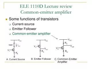
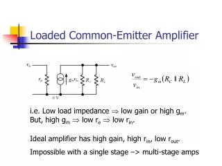
Loaded Common-Emitter Amplifier. i.e. Low load impedance Þ low gain or high g m . But, high g m Þ low r e Þ low r in . Ideal amplifier has high gain, high r in , low r out . Impossible with a single stage –> multi-stage amps. Example – An Operational Amplifier. Differential Amp.

Loaded Common-Emitter Amplifier
E N D
Presentation Transcript
Loaded Common-Emitter Amplifier i.e. Low load impedance Þ low gain or high gm. But, high gmÞ low reÞ low rin. Ideal amplifier has high gain, high rin, low rout. Impossible with a single stage –> multi-stage amps
Example – An Operational Amplifier Differential Amp Voltage Amp Power Amp + -
Power Amplifier Stages Properties : • Low voltage gain (usually unity). • High current gain. • Low output impedance. • High input impedance.
Power Amplifier Designs Differences between power amplifier designs : • Efficiency / Power dissipation. • Complexity / Cost. • Linearity / Distortion. Power amplifier designs are usually classified according to their conduction angle. (More on this later)
Efficiency / Dissipation The efficiency, h, of an amplifier is the ratio between the power delivered to the load and the total power supplied: Power that isn’t delivered to the load will be dissipated by the output device(s) in the form of heat.
Complexity / Cost • If you want a cheap simple solution, you ideally want: • Low component count (fewer transistors) • Easy design (no hard sums) • Easy set-up / calibration • Of course, this probably won’t be the case for the best power amplifiers
Linearity / Distortion • For an ideal power amplifier: • The voltage gain is unity • The output voltage exactly equals the input voltage • For real power amplifiers: • The voltage gain is slightly less than one • The input-output relationship might not be perfectly linear • Other sources of distortion can be present (e.g. cross-over distortion) • Non-linearity causes harmonic distortion which, if large enough, can be audible and annoying
Amplifier Classes: Conduction Angle The conduction angle gives the proportion of an a.c. cycle which the output devices conduct for. E.g. On all the time Þ 360 ° On half the time Þ 180 ° etc.
Class A Operating Mode Iout Time One device conducts for the whole of the a.c. cycle. Conduction angle = 360 °.
Class B Operating Mode Iout Time Two devices conduct for half of the a.c. cycle each. Conduction angle = 180 °.
Class AB Operating Mode Iout Time Two devices conduct for just over half of the a.c. cycle each. Conduction angle > 180 ° but << 360 ° .
Class C Operating Mode Iout Time One device conducts a small portion of the a.c. cycle. Conduction angle << 180 °.
Class D Operating Mode Iout Time Each output device always either fully on or off – theoretically zero power dissipation.
Differences Between Classes • Class A : Linear operation, very inefficient. • Class B : High efficiency, non-linear response. • Class AB : Good efficiency and linearity, more complex than classes A or B though. • Class C : Very high efficiency but requires narrow band load. • Class D : Potentially very high efficiency but requires low pass filter on load.
Summary • Multi-stage amplifiers generally consist of a voltage gain stage and a current gain (or power amplifier) stage. • Several operating modes for power amplifiers can be designed. • Major differences between modes are efficiency, complexity and linearity.