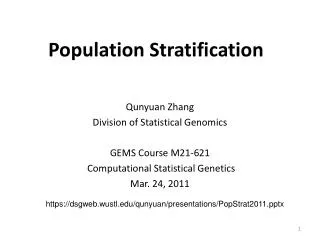
Population stratification
Population stratification. Background & PLINK practical. Variation between, within populations. Any two humans differ ~0.1% of their genome (1 in ~1000bp) ~8% of this variation is accounted for by the major continental racial groups Majority of variation is within group


Population stratification
E N D
Presentation Transcript
Population stratification Background & PLINK practical
Variation between, within populations • Any two humans differ ~0.1% of their genome (1 in ~1000bp) • ~8% of this variation is accounted for by the major continental racial groups • Majority of variation is within group • but genetic data can still be used to accurately cluster individuals • although biological concept of “race” in this context controversial
Stratified populations: Wahlund effect Sub-population 1 2 A1 0.1 0.9 A2 0.9 0.1 A1A1 0.01 0.81 A1A2 0.18 0.18 A2A2 0.81 0.01 1+2 0.5 0.5 0.41 (0.25) 0.18 (0.50) 0.41 (0.25)
Quantifying population structure • Expected average heterozygosity • in random mating subpopulation (HS) • in total population (HT) • from the previous example, • HS = 0.18 , HT = 0.5 • Wright’s fixation index • FST = ( HT - HS ) / HT • FST = 0.64 • 0.01 - 0.05 for European populations • 0.1 - 0.3 for most divergent populations
Male/female acceptance rate • Confounding due to unmeasured variables is a common issue in epidemiology • “Simpson’s paradox” • Berkley sex bias case • claim that female graduate applicants were prejudiced against • 44% men accepted, 35% women • but, stratified by department, no intra-department differences (see figure) • i.e. women more likely to apply to departments that were harder to get into (for both males and females) • In genetic association studies, • “accepted or not” disease or not • “male/female” genetic variant • “department” ancestry • Happens when both outcome and genotype frequencies vary between different ethnic groups in the sample Department Of all applicants, % female Department
Approaches to detecting stratification using genome-wide SNP data • Genomic control • average correction factor for test statistics • ratio of median chi-sq to expectation under null (0.456 for 1df) • Clustering approaches • assign individuals to groups • model based and distance based • Principal components analysis, multidimensional scaling • continuous indices of ancestry
2 Stratification adjust test statistic Genomic control 2 No stratification Test locus Unlinked ‘null’ markers
Structured association LD observed under stratification Unlinked ‘null’ markers Subpopulation A Subpopulation B
Discrete subpopulation model • K sub-populations, “latent classes” • Sub-populations vary in allele frequencies • Random mating within subpopulation • Within each subpopulation • Hardy-Weinberg and linkage equilibrium • For population as a whole • Hardy-Weinberg and linkage disequilibrium
Worked example • Look at Excel spreadsheet ~pshaun/pop-strat.xls • Scenario: two sub-populations, of equal frequency in total population. We know allele frequencies for 5 markers unlinked markers • Problem: For a given individual with genotypes on these 5 markers, what is the probability of belonging to population 1 versus population 2? • Allele frequencies: Steps: 1) Class-specific allele frequencies class-specific genotype frequencies (HWE) 2) Single locus multi-locus (5 marker) genotype frequencies (LE), P(G|C) 3) Prior probability of class, P(C). Hint: we are given this above. 4) Bayes theorem to give P(C|G) from P(G|C) and P(C)
Statistical approaches to uncover hidden population substructure • Goal : assign each individual to class C of K • Key : conditional independence of genotypes, G within classes (LE, HWE) P(C) prior probabilities P(G | C) class-specific allele/genotype frequencies P(C | G) posterior probabilities Bayes theorem: Problem: in practice, we don’t know P(G|C) or P(C) either! Solution: EM algorithm (LPOP), or Bayesian approaches (STRUCTURE) Sum over j = 1 to K classes
E-M algorithm E step: counting individuals and alleles in classes P(C) -2LL P(C | G) P(G |C) Converged? M step: Bayes theorem, assume conditional independence
Stratification analysis in PLINK • Calculate IBS sharing between all pairs • “--genome” command; can take long time, but can be parallelized easily • generates (large) .genome file • can be used to spot sample duplicates • also contains IBD estimates: these are only meaningful within a ~homogeneous sample • Given IBS data, perform clustering • complete linkage clustering • can specify various constraints, e.g. PPC test, cluster size (e.g. 1:1 matching) or # of clusters • Given IBS data, perform MDS • extract first K components, e.g.4-6 • plot each component, each pair of components
Han Chinese Japanese Multidimensional scaling/PCA Pairwise allele-sharing metric Reference Same population Different population Hierarchical clustering
Distribution of IBS between and within HapMap subpopulations YRI/CEU YRI/CHB YRI/JPT CEU/CHB CEU/JPT YRI CEU CHB JPT CHB/JPT CEU (P/O) YRI (P/O)
Multidimensional scaling (MDS) analysis HapMap data (equiv. to PCA) CEPH/European Yoruba Han Chinese Japanese ~2K SNPs
Han Chinese Japanese ~10K SNPs
PPC (pairwise population concordance) test {AA,BB} : {AB,AB} 1 : 2 { individual 1 , individual 2 } Expected 1:2 ratio in individuals from same population Significance test of a binomial proportion Note: Requires analysis to be of subset of SNPs in approx. LE within sub-population. Would also be sensitive to inbreeding
Two example pairs: (50K SNPs with 100% genotyping) 1 HCB1 HCB8 HCB26 HCB5 HCB15 2 HCB2 HCB45 HCB12 3 HCB3 HCB14 HCB32 HCB18 HCB27 HCB23 HCB30 4 HCB4 HCB38 HCB39 HCB20 5 HCB6 HCB21 HCB43 6 HCB7 HCB29 HCB31 HCB11 HCB40 HCB24 HCB33 7 HCB9 HCB16 HCB22 8 HCB10 HCB44 HCB19 HCB41 HCB42 HCB35 HCB36 9 HCB13 HCB17 HCB34 HCB25 HCB28 HCB37 10 JPT1 JPT19 JPT13 JPT16 JPT29 JPT36 11 JPT2 JPT28 12 JPT3 JPT17 JPT38 JPT44 JPT8 JPT23 13 JPT4 JPT18 JPT21 JPT27 JPT41 JPT43 14 JPT5 JPT30 JPT39 JPT42 JPT9 15 JPT6 JPT37 JPT24 16 JPT7 JPT12 JPT10 JPT25 JPT14 JPT26 JPT34 JPT33 17 JPT11 JPT31 JPT40 JPT15 JPT22 18 JPT20 19 JPT32* 20 JPT35 Proportion of all CHB-CHB pairs significant = 0.076 Proportion of all CHB-JPT pairs significant = 0.475 (Power for difference at p=0.05 level)
MDS analysis • Often useful to treat each MDS component as a QT and perform WGAS (regress it on all SNPs), to ask: • what is the genomic control lambda? If not >>1, then the component probably does not represent true, major stratification • which genomic regions load particularly strongly on the component (i.e. which regions show largest frequency differences between the groups the component is distinguishing?)
Practical example: bipolar GWAS CONTROLS CASES USA UK Evaluated via permutation that within site the average case is equally similar to the average control as another case
Fine-scale genetic variation reflects geography Novembre et al, Nature (2008)