Nonlinear Dynamical Invariants for Speech Recognition
240 likes | 260 Vues
Explore the robustness of speech recognition through nonlinear dynamical invariants capturing key information from speech signals, beyond traditional measures. Study attractors, chaos, Lyapunov exponents, and more. Utilize reconstructed phase space methods for system characterization.

Nonlinear Dynamical Invariants for Speech Recognition
E N D
Presentation Transcript
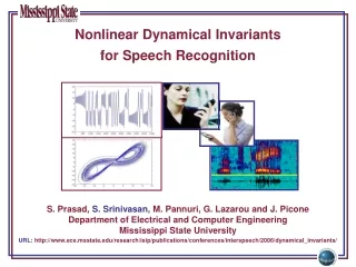
Nonlinear Dynamical Invariantsfor Speech Recognition S. Prasad, S. Srinivasan, M. Pannuri, G. Lazarou and J. Picone Department of Electrical and Computer Engineering Mississippi State University URL:http://www.ece.msstate.edu/research/isip/publications/conferences/interspeech/2006/dynamical_invariants/
Motivation • State-of-the-art speech recognition systems relying on linear acoustic models suffer from robustness problem. • Our goal: To study and use new features for speech recognition that do not rely on traditional measures of the first and second order moments of the signal. • Why nonlinear features? • Nonlinear dynamical invariants may be more robust (invariant) to noise. • Speech signals have both periodic-like and noise-like segments – similar to chaotic signals arising from nonlinear systems. • The motivation behind studying such invariants: to capture the relevant nonlinear dynamical information from the time series – something that is ignored in conventional spectral analysis.
Attractors for Dynamical Systems • System Attractor: Trajectories approach a limit with increasing time, irrespective of the initial conditions within a region • Basin of Attraction: Set of initial conditions converging to a particular attractor • Attractors: Non-chaotic (point, limit cycle or torus),or chaotic (strange attactors) • Example: point and limit cycle attractors of a logistic map (a discrete nonlinear chaotic map)
Strange Attractors • Strange Attractors: attractors whose shapes are neither points nor limit cycles. They typically have a fractal structure (i.e., they have dimensions that are not integers but fractional) • Example: a Lorentz system with parameters
Characterizing Chaos • Exploit geometrical (self-similar structure) aspects of an attractor or the temporal evolution for system characterization • Geometry of a Strange Attractor: • Most strange attractors show a similar structure at various scales, i.e., parts are similar to the whole. • Fractal dimensions can be used to quantify this self-similarity. • e.g., Hausdorff, correlation dimensions. • Temporal Aspect of Chaos: • Characteristic exponents or Lyapunov exponents (LE’s) - captures rate of divergence (or convergence) of nearby trajectories; • Also Correlation Entropy captures similar information. • Any characterization presupposes that phase-space is available. • What if only one scalar time series measurement of the system (and not its actual phase space) is available?
Reconstructed Phase Space (RPS): Embedding • Embedding: A mapping from a one-dimensional signal to an m-dimensional signal • Taken’s Theorem: • Can reconstruct a phase space “equivalent” to the original phase space by embedding with m ≥ 2d+1 (d is the system dimension) • Embedding Dimension: a theoretically sufficient bound; in practice, embedding with a smaller dimension is adequate. • Equivalence: • means the system invariants characterizing the attractor are the same • does not mean reconstructed phase space (RPS) is exactly the same as original phase space • RPS Construction: techniques include differential embedding, integral embedding, time delay embedding, and SVD embedding
Reconstructed Phase Space (RPS): Time Delay Embedding • Uses delayed copies of the original time series as components of RPS to form a matrix • m: embedding dimension, : delay parameter • Each row of the matrix is a point in the RPS
Reconstructed Phase Space (RPS) Time Delay Embedding of a Lorentz time series
Lyapunov Exponents • Quantifies separation in time between trajectories, assuming rate of growth (or decay) is exponential in time, as: • where J is the Jacobian matrix at point p. • Captures sensitivity to initial conditions. • Analyzes separation in time of two trajectories with close initial points • where is the system’s evolution function.
Correlation Integral • Measures the number of points within a neighborhood of radius, averaged over the entire attractor as: • where are points on the attractor (which has N such points). • Theiler’s correction: Used to prevent temporal correlations in the time series from producing an underestimated dimension. • Correlation integral is used in the computation of both correlation dimension and Kolmogorov entropy.
Fractal Dimension • Fractals: objects which are self-similar at various resolutions • Correlation dimension: a popular choice for numerically estimating the fractal dimension of the attractor. • Captures the power-law relation between the correlation integral of an attractor and the neighborhood radius of the analysis hyper-sphere as: • where is the correlation integral.
Kolmogorov-Sinai Entropy • Entropy: a well-known measure used to quantify the amount of disorder in a system. • Numerically, the Kolmogorov entropy can be estimated as the second order Renyi entropy ( ) and can be related to the correlation integral of the reconstructed attractor as: • where D is the fractal dimension of the system’s attractor, d is the embedding dimension and is the time-delay used for attractor reconstruction. • This leads to the relation: • In a practical situation, the values of and are restricted by the resolution of the attractor and the length of the time series.
Kullback-Leibler Divergence for Invariants • Measures discrimination information between two statistical models. • We measured invariants for each phoneme using a sliding window, and built an accumulated statistical model over each such utterance. • The discrimination information between a pair of models and is given by: • provides a symmetric divergence measure between two populations from an information-theoretic perspective. • We use as the metric for quantifying the amount of discrimination information across dynamical invariants extracted from different broad phonetic classes.
Experimental Setup • Collected artificially elongated pronunciations of several vowels and consonants from 4 male and 3 female speakers • Each speaker produced sustained sounds (4 seconds long) for three vowels (/aa/, /ae/, /eh/), two nasals (/m/, /n/) and three fricatives (/f/, /sh/, /z/). • The data was sampled at 22,050 Hz. • For this preliminary study, we wanted to avoid artifacts introduced by coarticulation. • Acoustic data to reconstructed phase space: using time delay embedding with a delay of 10 samples. (This delay was selected as the first local minimum of the auto-mutual information vs. delay curve averaged across all phones. • Window Size: 1500 samples.
Experimental Setup (Tuning Algorithmic Parameters) • Experiments performed to optimize parameters (by varying the parameters and choosing the value at which we obtain convergence) of estimation algorithm. • Embedding dimension for LE and correlation dimension: 5 • For Lyapunov exponent: • number of nearest neighbors: 30, • evolution step size: 5, • number of sub-groups of neighbors: 15. • For Kolmogorov entropy: • Embedding dimension of 15
Tuning Results: Lyapunov Exponents Lyapunov Exponents • For vowel: /ae/ For nasal: /m/ For fricative: /sh/ • In all three cases, the positive LE stabilizes at an embedding dimension of 5. • Positive LE much higher for fricative than nasals and vowels.
Tuning Results: Kolmogorov Entropy Kolmogorov Entropy • For vowel: /ae/ For nasal: /m/ For fricative: /sh/ • For vowels and nasals: Have stable behavior with embedding dimensions around 12-15. • For fricatives: Entropy estimate consistently increases with embedding dimension.
Tuning Results: Correlation Dimension Correlation Dimension • For vowel: /ae/ For nasal: /m/ For fricative: /sh/ • For vowels and nasals: Clear scaling region at epsilon = 0.75; Less sensitive to variations in embedding dimensions from 5-8. • For fricatives: No clear scaling region; more sensitive to variations in embedding dimension.
Experimental Results : KL Divergence - LE • Discrimination information for: • vowels-fricatives: higher • nasals-fricatives: higher • vowels-nasals: lower
Experimental Results : KL Divergence – Kolmogorov Entropy • Discrimination information for: • vowels-fricatives: higher • nasals-fricatives: higher • vowels-nasals: lower
Experimental Results : KL Divergence – Correlation Dimension • Discrimination information for: • vowels-fricatives: higher • nasals-fricatives: higher • vowels-nasals: lower
Summary and Future Work • Conclusions: • Reconstructed phase-space from speech data using Time Delay Embedding. • Extracted three nonlinear dynamical invariants (LE, Kolmogorov entropy, and Correlation Dimension) from embedded speech data. • Demonstrated the between-class separation of these invariants across8 phonetic sounds. • Encouraging results for speech recognition applications. • Future Work: • Study speaker variability with the hope that variations in the vocal tract response across speakers will result in different attractor structures. • Add these invariants as features for speech and speaker recognition.
Pattern Recognition Applet: compare popular linear and nonlinear algorithms on standard or custom data sets • Speech Recognition Toolkits: a state of the art ASR toolkit for testing the efficacy of these algorithms on recognition tasks • Foundation Classes: generic C++ implementations of many popular statistical modeling approaches • Resources
References • Kumar, A. and Mullick, S.K., “Nonlinear Dynamical Analysis of Speech,” Journal of the Acoustical Society of America, vol. 100, no. 1, pp. 615-629, July 1996. • Banbrook M., “Nonlinear analysis of speech from a synthesis perspective,” PhD Thesis, The University of Edinburgh, Edinburgh, UK, 1996. • Kokkinos, I. and Maragos, P., “Nonlinear Speech Analysis using Models for Chaotic Systems,” IEEE Transactions on Speech and Audio Processing, pp. 1098- 1109, Nov. 2005. • Eckmann, J.P. and Ruelle, D., “Ergodic Theory of Chaos and Strange Attractors,” Reviews of Modern Physics, vol. 57, pp. 617‑656, July 1985. • Kantz, H. and Schreiber T., Nonlinear Time Series Analysis, Cambridge University Press, UK, 2003. • Campbell, J. P., “Speaker Recognition: A Tutorial,” Proceedings of IEEE, vol. 85, no. 9, pp. 1437-1462, Sept. 1997.
