Building a model (three more aspects)
Workshop on Statistical modelling with SAS – part II . Building a model (three more aspects). Dragos Calitoiu, Ph.D. Hasan Mytkolli, Ph.D. June 22, 2009.

Building a model (three more aspects)
E N D
Presentation Transcript
Workshop on Statistical modelling with SAS – part II Building a model (three more aspects) Dragos Calitoiu, Ph.D. Hasan Mytkolli, Ph.D. June 22, 2009 Hasan Mytkolli and Dragos Calitoiu are modellers for Bank of America – Canada Card Services. Opinions, ideas, and everything said in this presentation are of the authors and should not be confounded with their Position in the Bank. Hasan Mytkolli and Dragos Calitoiu are also members of CORS (Canadian Operational Research Society) and OPTIMOD Research Institute. Contact: Hasan.Mytkolli@mbna.com and Dragos.Calitoiu@mbna.com
The content of this presentation • Finding the best subset of variables for a model; • Checking for normality; • The rationale of variable transformations.
Finding the best subset of variables • Statistical model: - a set of mathematical equations which describe the behavior of an object of study in terms of random variables and of their associated probability distributions. - a probability distribution that uses observed data to approximate the true distribution of probabilistic events • The mystery in building a statistical model is that the true subset of variables defining theperfectmodel is not known. The goal: to fit a parsimonious model that explains variation in the dependent variable with a small set of predictors, as accurately as possible. • True vs. parsimonious model ; • Perfect vs. as accurately as possible.
Finding the best subset of variables Observation True distribution Data Approximation Estimation Statistical Model For example: In fitting a regression model, we want to detect the “true set of explanatory variables”. However, due to computational constraints or business constraints, we want to use only 10-15 variables as the “true set”. Which ones?
Finding the best subset of variables • When the variables are not correlated with each other (rare): we can assess a variable’s unique contribution and rank the variables. • When the variables are correlated with each other (often): - we can assess a variable’s relative importance with respect to the presence of other variables. - the variables interact with each other such that their total effect on the model’s prediction is greater than the sum of their individual effects. - the Wald chi-square (in the case of logistic regression) is an indicator of a variable’s relative importance and of selecting the best subset.
Finding the best subset of variables ( the case of logistic regression) Selecting the best subset process: • If you have the dataset, use your experience as a guide to identify all of the useful variables. Occasionally, you can build new variables (ratio, min, max, aggregate). • If there are too many variables, run a “survey” and produce a starter set. • Perform logistic regression analysis on the starter set; delete one or two variables with minimum Wald chi-square. After deleting, the order of the remaining variables can change. The greater the correlation between the remaining variables, the greater the uncertainty of declaring important variables. • Eliminate correlations.
Finding the best subset of variables (the case of logistic regression) Selecting the best subset: • If you have the dataset, use your experience as a guide to identify all of useful variables. • If there are too many variables, run a “survey” and produce a starter set. • Perform logistic regression (automated procedure): - Backward Elimination (Top down approach); - Forward Selection (Bottom up approach); - Stepwise Regression (Combines Forward/Backward). • Eliminate correlations: - correlation; - variance inflation factor (VIF) ; - multicollinearity.
Finding the best subset of variables: “the survey” %let varlist= var1 var2 var3 var4 var5; %macro var_filt(inputfile, depend_var, nboots, bootsize, slent, slst, outfile); %do i=1 %to &nboots; proc surveyselect method=srs data=&inputfile out=boot&i seed=%sysevalf(1000+&i*10) n=&bootsize; run; proc logistic data=boot&i desc noprint outest=log_var_filt_&i ; model &depend_var=&varlist / selection=stepwise slentry=&slent slstay=&slst; run; proc datasets nolist; append data=log_var_filt_&i base= &outfile force; run; %end; %mend var_filt; options mprint mlogic spool; %var_filt(file_name, dep_var, 20, 30000, 0.2, 0.1, file_output);
Finding the best subset of variables: “the survey” %let varlist= var1 var2 var3 var4 var5;/* enter all the variables here */ %macro var_filt(inputfile, depend_var, nboots, bootsize, slent, slst, outfile); %do i=1 %to &nboots; /* run the stepwise logistic regression nboots time */ proc surveyselect method=srs data=&inputfile out=boot&i seed=%sysevalf(1000+&i*10) /* generate randomly a small data set for each run */ n=&bootsize; run; proc logistic data=boot&i desc noprint outest=log_var_filt_&i ; model &depend_var=&varlist / selection=stepwise slentry=&slent /* the threshold of entering a variable into the model */ slstay=&slst; /* the threshold of leaving the model */ run; proc datasets nolist; append data=log_var_filt_&i base= &outfile force; /* append all the output files */ run; %end; %mend var_filt; options mprint mlogic spool; %var_filt(file_name, dev_var, 20, 30000, 0.2, 0.1, file_output); ods html file='var_selection.html'; title 'Variable Selection Logistic'; proc means data=file_output n; run; title; ods html close;
Finding the best subset of variables: “the survey” Example - the output of the survey : From a set of 460 variables, only 28 entered into the survey (namely they are independent variables in stepwise regressions). We decided to use only 14 of them (with the frequency greater than 10 out of 30 runs). Remark: this is ONLY an example. Usually, we can continue to work with circa 40 variables, after this survey.
Finding the best subset of variables (the case of logistic regression) Selecting the best subset: • If you have the dataset, use your experience as a guide to identify all of useful variables. • If there are too many variables, run a “survey” and produce a starter set. • Perform logistic regression (automated procedure): - Backward Elimination (Top down approach); - Forward Selection (Bottom up approach); - Stepwise Regression (Combines Forward/Backward). • Eliminate correlations: - correlation; - variance inflation factor (VIF) ; - multicollinearity.
Finding the best subset of variables: Correlation proc corr data=filename; var var1 = var2 …varN; run; - This procedure computes the Pearson correlation coefficient and produces simple descriptive statistics (mean, standard deviation sum, minimum and maximum ) for all pairs of variables listed in the VAR statement. - It also computes a p-value for testing whether the true correlation is zero. - The correlations are given in matrix form. - A correlation of more than 0.7 between 2 variables encourages deleting one of the variables. Use experience and the Wald chi-square for identifying which one to delete.
Finding the best subset of variables: VIF (variation inflation factor) proc reg data=filename; model var1 = var2 …varN/vif; run; - Measure of how highly correlated each independent variable is with the other predictors in the model. Used to identify multicollinearity. - Values larger than 10 for a predictor imply large inflation of standard errors for regression coefficients due to this variable being in the model. - Inflated standard errors lead to small t-statistics for partial regression coefficients and wider confidence intervals.
Finding the best subset of variables: Multicollinearity proc reg data=filename; model var1 = var2 …varN/collin; run; - For no collinearity between variables, the condition index must be less than 10. - If this condition is not satisfied, you can find a pair where the proportion of variation is greater than 0.7. You have to eliminate one variable from that pair. Remark: The intercept can be one member of the pair. You will delete the second member. You can conclude that a variable highly correlated with the intercept has a vary small variance, namely it is almost constant.
Finding the best subset of variables for the model How many variables? • A too small set of variables: a poor predicting response. • Overfitted model (too many variables): a “too perfect” picture of the development data set (memorization) instead of capturing the desired pattern from the entire data set. Capitalizing on the idiosyncrasies of the training data. • A well-fitted model is typically defined by a handful of variables because it does not include “idiosyncracy” variables.
Finding the best subset of variables for the logistic model How good is a model? Hirotugu Akaike (1971): AIC (Akaike’s Information Criterion) - Based on entropy, information and likelihood. Informational statistical modelling: - Information criteria are used to estimate expected entropy (analogous to expected uncertainty in the data) by taking simultaneously into account both the “goodness-of-fit” of the model and the complexity of the model required to achieve that fit. - Model complexity involves both the number of parameters and the interaction (correlation) between them.
Testing for normality • One of the critical steps in data analysis is checking for normality, in order to make assumptions about the distributions of the data. • If the specified distributional assumption about the data is not valid, the analysis based on this assumption can lead to incorrect conclusions.
Testing for normality • Skewness: the standardized 3rd central moment of a distribution; • Positive skewness indicates a long right tail; • Negative skewness indicates a long left tail; • Zero skewness indicates symmetry around the mean; • Kurtosis: the standardized 4th central moment of a distribution; • The kurtosis for the normal distribution is 3; • Positive excess kurtosis indicates flatness (long, fat tails); • Negative excess kurtosis indicates peakedness;
Testing for normality • We used three well-known tests for rejecting the normality hypothesis, namely: • Kolmogorov-Smirnov (K-S) test; • Anderson-Darling test; • Cramer-von Mises test. G. Peng, Testing Normality of Data using SAS , PharmaSUG 2004, May 22-26, 2004, San Diego, California.
Testing for normality 1. Kolmogorov-Smirnov test : • based on the empirical distribution function (EDF).; • K-S D is the largest vertical distance between the distribution function F(x) and the EDF(F(x)) which is a step function that takes a step of height 1/n at each observation; • to test normality, the K-S D is computed using the data set against a normal distribution with mean and variance equal to the sample mean and variance. 2. Anderson-Darling test : • uses the quadratic class EDF, based on the squared difference (F(n)-F(x)^2 ; • gives more weights to the tails than does the K-S test, the former being more sensitive to the center of the distribution than at the tails; • The procedure of emphasizing the tails is done by setting a function weighting the square difference. 3. The Cramer-von Mises test : • also based on the quadratic class of EDF; • however, the weight function in this scenario is considered equal to unity. The last two tests describe better the entire data set from the sum of the variances point of view. The K-S test is much sensitive to the anomalies in the sample.
Testing for normality • SAS has implemented the commonly used normality tests in PROC UNIVARIATE. procunivariate data=name normal plot vardef=df; var name; • The normal option computes the three tests of the hypothesis that the data comes from a normal population. The p-value of the test is also printed. • The vardef= option specifies the divisor used in computing the sample variance. • vardef=df, the default, uses the degrees of freedom n-1; • vardef=n uses the sample size n. An alternative procedure is PROC CAPABILITY.
Testing for normality • For the left graph: mean 992.18, std 994.70.,skewness 1.53, kurtosis 3.29; • For the right graph: mean 5.50, std 2.87, skewness -9.29E-7, kurtosis -1.22; • For the normal distribution: skewness = 0, kurtosis = 3.
Data transformation is one of the remedial actions that may help to make data normal. The rationale of variable transformations. To reduce variance; To transform optimally the information content hidden in data. Transforming data
A method of re-expressing variables to straighten a relationship between two continuous variables, say X and Y. Examples are: 1/x² reciprocal of square (power -2); 1/x reciprocal (power -1); x0=ln(x) natural logarithm; x½ square root (power 0.5); x² square (power 2). Transforming data: Ladder of Powers and Bulging Rule Y2 and/or X-1/2 Y2 and/or X2 • Going up-ladder of powers: raising a variable to a power greater than 1: X2, X3…or Y2 ,Y3… • Going down-ladder of powers: raising a variable to a power less than 1: X1/2 ,X0, X-1/2 or Y1/2, Y0,Y-1/2 • Remarks: Not so much freedom with the dependent variable ; if you have Y=f(X1,X2) you cannot do Y1/2=G(X1) and Y0=H(X2); Y0 and/or X-1/2 Y-2 and/or X2
George Box and David Cox developed a procedure to identify an appropriate exponent (λ) to transform data into a “normal shape”. The exponent λ indicates the power to which all data should be raised. The aim of the Box-Cox transformations is to ensure that the usual assumptions for the Linear Model hold, namely y ~N(Xβ, σ2In). The original form for Box-Cox (1964): The Box-Cox Transformations Practically, the algorithm searches from λ=-5 to λ=+5 with a step of 0.2 until the best value is found. • Weakness: Cannot be applied to negative numbers.
They proposed in the same paper an extension. Find λ2 such that y+λ2 >0 for any y. With this condition, the transformation can accommodate negative y’s: The Box-Cox Transformations (extended)
Yeo and Johnson (2000) proposed a new set of transformations for real numbers: Yeo and Johnson Transformations
options mlogic mprint ; /** This is the main macro code **/ /** Fileinput - is your data file **/ /** ul - is the upper limit for the power transformation **/ /** ll - is the absolute value of the lower limit for the power transformation **/ /** base - is the base choice or alternative to which other alternatives will compare to**/ /** dependent - is the dependent variable **/ /** independent - is the independent variable you are looking for transformation **/ %macro boot_box_cox(fileinput, bootvol, nrboots,dependent, independent, lowpower, highpower, step); data temp (keep=&dependent &independent); set &fileinput; run; proc datasets nolist; delete histo_data; run; %do i=1 %to &nrboots; proc surveyselect data=temp method=srs out=boot&i seed=%sysevalf(10000+&i*10) n=&bootvol; run; data tempi (rename=(&independent=x)); set boot&i; run; data tempi; set tempi; if (x<0) then do; %do k10=%sysevalf(0) %to %sysevalf(-&lowpower.*10) %by %sysevalf(&step.*10); k=%sysevalf(-&k10/10); y=(1-x); z=2-k; xk=((1-x)**(2-k)-1)/(k-2); output; %end; %do k10=%sysevalf(&step.*10) %to %sysevalf(&highpower.*10) %by %sysevalf(&step.*10); k=%sysevalf(&k10/10); %if %sysevalf(&k10.) = 20 %then %do; xk=-log(1-x); output; %end; %else %do; xk=((1-x)**(2-k)-1)/(k-2); output; %end; %end; end; else do; The code The search for finding the optimum exponent is done in the range of (-lowerpower, highpower) with a fixed step.
%do k10=%sysevalf(&step.*10) %to %sysevalf(-&lowpower.*10) %by %sysevalf(&step.*10); k=%sysevalf(-&k10/10); xk=((x+1)**k-1)/k; output; %end; k = 0; xk=log(x+1); output; %do k10=%sysevalf(&step.*10) %to %sysevalf(&highpower.*10) %by %sysevalf(&step.*10); k=%sysevalf(&k10/10); xk=((x+1)**k-1)/k; output; %end; end; label k='Box-Cox Power' ; run; proc sort data=tempi; by k; run; /** You have created all the transformed data ready for one-variable estimation **/ proc logistic data=tempi descending noprint outest=boot_k&i (keep=_name_ k _lnlike_); model &dependent= xk; by k; run; title; proc gplot data=boot_k&i; symbol1 v=none i=join; plot _lnlike_*k; title "BC Utilization likelihood - &independent i=&i "; run; title; proc sort data= boot_k&i ; by descending _lnlike_; run; data tempout; set boot_k&i ( obs=1); run; proc append base=histo_data data=tempout force;run; proc datasets nolist; delete tempi tempout boot&i boot_k&i ; run; %end; title4 "Frequency table for the B_C transformation: variable &independent"; proc freq data=histo_data ; tables k; run; title4 ; %mend boot_box_cox; %boot_box_cox(file_name, 50000, 20, var_dep, var_indep, -4, 4, 0.2); The code…
The output: the histogram and one file as example. rsubmit; proc gplot data=boot_k&i; symbol1 v=none i=join; plot _lnlike_*k; title "BC Utilization likelihood - &independent i=&i "; run; endrsubmit;
The output: the likelihood from one file (out of 20) The Box_Cox index is 0.4 in this example.
Summary • Finding the best subset of variables for a model; • Checking for normality; • The rationale of variable transformations. • QUESTIONS? • Contact: Hasan.Mytkolli@mbna.com and Dragos.Calitoiu@mbna.com