Download
1 / 48
480 likes | 651 Vues
Tropical Cyclone Overview: Lesson 3 Applications of Microwave Data. Introduction SSM/I algorithms Overview of the Advanced Microwave Sounder Unit (AMSU) Review of hydrostatic and dynamical balance approximations Experimental intensity/structure estimation algorithm. GOES Imager Channels :

E N D
Tropical Cyclone Overview: Lesson 3Applications of Microwave Data • Introduction • SSM/I algorithms • Overview of the Advanced Microwave Sounder Unit (AMSU) • Review of hydrostatic and dynamical balance approximations • Experimental intensity/structure estimation algorithm
GOES Imager Channels: Channel 1 - Visible - .6 µm ( .52- .72) Channel 2 - Shortwave IR - 3.9 µm (3.78- 4.03) Channel 3 - Water Vapor - 6.7 µm (6.47-7.02) Channel 4 - Longwave IR - 10.7 µm (10.2-11.2) Channel 5 - Split Window - 12.0 µm (11.5-12.5) SSM/I, AMSU Microwave Frequencies: 20-150 Ghz (1.5-0.2 cm) 1 2 3 4 5 Microwave
Special Sensor Microwave Imager (SSM/I) • Passive Microwave Imager on DMSP polar orbiting satellite • Conical Scan, 1400 km swath width • Four Frequencies, Horizontal and Vertical Polarization • 19.4 GHz (H,V), 22.2 GHz (V), 37.0 GHz (H,V), 85.5 GHz (H,V) • Note: Similar frequencies on TRMM satellite • Horizontal Resolution: 15-50 km • Senses below cloud-top
SSM/I Products/Applications • Vertically integrated water vapor, liquid • Rain rate • Sea Ice • Ocean Surface Wind Speed • 85 GHz ice scattering signal useful for tropical cyclone analysis • Highlights convectively active regions below cirrus canopy seen in IR imagery
A: B: C: A: Uses SSM/I Rain Rates B: AE uses GOES Longwave IR (Channel 4) C. GMSRA Combines all GOES channels
Ocean Surface Winds from SSM/I • Passive Microwave (SSM/I, TMI) • 19 GHz emissivity increases as capillary waves and sea foam are generated by wind • Rain, thick clouds degrade algorithm • Combine 19V GHz, 22V GHz, 37V GHz, 37H GHz • Winds limited to ~40 kt • Provides speed but not direction
Hurricane Jeanne 23 Sept 98 IR VIS 85 GHz Comp. (From NRL web-site).
Properties of NOAA-15 • Polar orbiting satellite • 833 km above earth’s surface • 14.2 revolutions per day • Launched May 13, 1998 (Vandenberg AFB) • Instrumentation: • AVHRR, HIRS, AMSU, SBUV • First in new series (NOAA-K,L,M) • NOAA-16 Launched Fall 2000
AMSU Instrument Properties • AMSU-A1 • 13 frequencies 50-89 GHz • 48 km maximum resolution • Vertical temperature profiles 0-45 km • AMSU-A2 • 2 frequencies 23.8, 31.4 GHz • 48 km maximum resolution • Precipitable water, cloud water, rain rate • AMSU-B (interference problems) • 5 frequencies: 89-183 GHz • 16 km maximum resolution • Water vapor soundings
Hurricane Mitch AVHRR Image 27 October 1998 NOAA-15 Corresponding AMSU-B 89 GHz
AMSU-A Moisture Algorithms • Total Precipitable Water (V) • V = cos() * f[TB(23.8),TB(31.4)] • Cloud Liquid Water (Q) • Q = cos( ) * g[TB(23.8),TB(31.4)] • Rain Rate (R) • R = 0.002 * Q 1.7 • Tropical Rainfall Potential (TRaP) • TRaP = Ra * D/c • Ra = avg. rain rate, D=storm dia., c = Storm Speed
AMSU-A Rainfall Rate for Hurricane Georges (.01 inches/hr) TRaP for Key West = 6.7 inches
Temperature Retrieval Algorithm • 15 AMSU-A channels included • Radiances adjusted for side lobes before conversion to brightness temperatures (BT) • BT adjusted for view angle • Statistical algorithm converts from BT to temperature profiles • 40 vertical levels 0.1-1000 mb • RMS error 1.0-1.5 K compared with rawindsondes
IR Imagery March 1, 1999 AMSU Temperature Retrieval (570 mb)
AMSU Tropical Cyclone Applications • Input for numerical models • Direct assimilation of AMSU radiances • Rain rate product input to physical initialization procedures • Apply hydrostatic/dynamical balance constraints to obtain height/wind fields • Height/winds input for intensity/structure intensity estimation technique
Hydrostatic Balance • Approximation to vertical momentum equation • Valid for horizontal scales > 10 km • dP/dz = -gP/RTv (Height coordinates) • P=pressure, z=height, Tv=virtual temperature • G=gravitational constant, R=ideal gas constant • Allows calculation of pressure as a function of height P(z), given temperature and moisture profile • d/dp = -RTv/P (Pressure coordinates) • Allows calculatation of geopotential height as a function of pressure (P) • Both forms require boundary conditions • Integration can be upwards or downwards • Contribution from moisture is fairly small and will be neglected (Tv replaced by T)
Dynamical Balance Conditions Provides Diagnostic Relationship Between Height and Wind • High latitude, synoptic-scale flows • Geostrophic balance • Axisymmetric flows • Gradient balance • Higher-order approximation to the divergence equation • Charney balance equation
Gradient Balance • Start with horizontal momentum equations in cylindrical/pressure coordinates • Assume no variation in the azimuthal direction • Radial momentum equation reduces to: V2/r + fV = d/dr V = tangential wind, r = radius f = Coriolis parameter = geopotential height from hydrostatic equation
Charney Nonlinear Balance Equation • NBE reduces to gradient wind in axisymmetric case • NBE reduces to geostrophic wind in low-amplitude case
Balance Winds from AMSU Data • Start with Advanced Microwave Sounder Unit (AMSU) data from NOAA-15 • Apply NESDIS statistical retrieval algorithm to get T from radiances • Use hydrostatic equation to get height field • NCEP analysis for lower boundary condition • Apply gradient (2-D) or Charney (3-D) balance to get winds • NCEP analysis for lateral boundary condition
2-D AMSU Wind Retrieval:Solution of the Gradient Wind Equation • Gradient Wind Equation: V2/r + fV = r • Find from V: = (V2/r + fV )dr • Find V from : V = -fr/2 ± [(fr/2)2 + r r]1/2 • Requires choice of root and [(fr/2)2 + r r] > 0
2D Analyses - Hurricane Gert Hydrometeor Corrected Temperature(r,z) Sfc Pressure (x,y) Tangential Wind(r,z) Uncorrected
Correction for Attenuation by Cloud Liquid Water and Ice Scattering • Use data base of 120 cases from 1999 hurricane season • Derive statistical correction to temperature as a function of CLW for P < 300 hPa • Identify isolated cold anomalies related to ice scattering using threshold technique • “Patch” cold regions using Laplacian filter from surrounding data
2-D AMSU Wind Retrieval Results • >250 cases analyzed in Atlantic and East Pacific basins during 1999-2000 • Inner core winds not resolved due to limited AMSU-A spatial resolution • Statistical relationship between AMSU analyses and intensity • Large differences in storm sizes • Useful for wind radii estimation • Analyses appear to capture vertical structure changes • 2-D analysis algorithm available for evaluation in West Pacific
Isaac 092800 120 kt Joyce 092700 70 kt AMSU 2-D Winds For Large and Small Storms
Low-Shear High-Shear AMSU 2-D Winds In Low-Shear and High-Shear Storm Environments. (Note the deeper cyclonic flow in the low-shear cases.)
Statistical Intensity Estimation • AMSU resolution prevents direct measurement of inner core • Correlate parameters from AMSU analyses with observed storm intensity • AMSU Predictors from 1999 storm sample: • r=600 to r=0 km pressure drop • Max tangential wind at 0 and 3 km • Max upper-level temperature anomaly • Average cloud-liquid water • Algorithm explains 70% of variance • Algorithm will be tested on 2000 data
Predicted vs. Observerd Maximum Winds(Preliminary Results with Dependent Data)
Statistical Size Estimation • Correlate parameters from AMSU analyses with observed storm size • Average radius of 34, 50 and 64 kt winds • AMSU Predictors from 1999 storm sample: • R=600 to r=0 km pressure drop • Max tangential wind at 0 and 3 km • Storm latitude • Estimated maximum wind • Average cloud-liquid water • Algorithm explains ~80% of variance • Algorithm will be tested on 2000 data
Predicted vs. Observed 34 kt Wind Radius(Preliminary Results with Dependent Data)
3-D AMSU Wind Retrieval:Charney Nonlinear Balance Equation • Charney balance equation: • 2 = -[(ux)2 +2vxuy + (vy)2] + f - u • For nondivergent flow: u=-y, v= x, = 2 • 2 = -2(xy)2 + 2(xx yy) + f 2 + y • Find from u,v: Poisson equation • Requires boundary values for • Find u,v from : Monge-Ampere Equation • Requires boundary values for u,v (or ) • Ellipticity condition: 2 + 1/2f2 > 0 • Possibility of two solutions
Charney Balance Equation Iterative Solution • Developed for early NWP models • Write balance equation as: 2 + f - [(ux)2+ (vx)2 + (uy)2 + (vy)2 + u+ 2] = 0 2 + f - [N ] = 0 where = 2 u = -y v= x • Solve for : = -(f/2) ± [(f/2)2 + N]1/2 • N = N() so iteration is necessary
Charney Balance Equation Variational Solution • Iterative method sometimes fails for tropical cyclone case • Variational solution method: • Define cost function as square of balance equation integrated over domain of interest • Add smoothness penalty term to cost function • Find u,v to minimize cost function • Minimization requires cost function gradient, determined from adjoint of balance equation • Boundary conditions for u,v from NCEP analysis
AMSU 850 hPa height First guess wind: (Ñ2u=0, Ñ2v=0) Nonlinear balance wind Balance Equation Variational Solution - Hurricane Floyd
Hurricane Floyd 850 mb Isotachs (kt) -80 -60 -40 -20 0
AMSU RECON Evaluation of AMSU Winds
Summary of Lesson 3 • Passive microwave data can penetrate through cloud tops • Data available from DMSP(SSM/I), NOAA-15/16 (AMSU), and TRMM (TMI) satellites • Algorithms available for ocean surface wind speed, integrated water content, rainfall rate, sea ice/snow cover • Data useful for qualitative analysis of tropical cyclone structure (banding, eye wall, etc) • AMSU temperature sounding can be combined with hydrostatic/dynamical balance constraints for tropical cyclone analysis