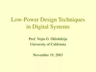
Low-Power Design Techniques in Digital Systems
990 likes | 1.66k Vues
Low-Power Design Techniques in Digital Systems. Prof. Vojin G. Oklobdzija University of California. Outline of the Talk. Power trends in VLSI Scaling theory and predictions Research efforts in power reduction Efficiency measures and design guidelines Latches and Flip-Flops for Low-Power

Low-Power Design Techniques in Digital Systems
E N D
Presentation Transcript
Low-Power Design Techniques in Digital Systems Prof. Vojin G. Oklobdzija University of California
Outline of the Talk • Power trends in VLSI • Scaling theory and predictions • Research efforts in power reduction • Efficiency measures and design guidelines • Latches and Flip-Flops for Low-Power • Dual-Edge FFs • SOI • Conclusion: Low-Power perspective
CMOS Circuits dissipate little power by nature”. So believed circuit designers (Kuroda-Sakurai, 95) 100 x4 / 3years 10 Power (W) 1 0.1 0.01 80 85 90 95 “By the year 2000 power dissipation of high-end ICs will exceed the practical limits of ceramic packages, even if the supply voltage can be feasibly reduced.” (* Taken from Sakurai’s ISSCC 2001 presentation)
Gloom and Doom predictions Source: Shekhar Borkar, Intel
Power versus Year:taken from ISSCC, uP Report, Hot-Chips High-end growing at 25% / year RISC @ 12% / yr X86 @ 15% / yr Consumer (low-end) At 13% / year
VDD, Power and Current Trend 2.5 200 500 Voltage 2 Power 1.5 Voltage [V] Power per chip [W] Current VDD current [A] 1 0.5 0 0 0 1998 2002 2006 2010 2014 Year International Technology Roadmap for Semiconductors 1999 update sponsored by the Semiconductor Industry Association in cooperation with European Electronic Component Association (EECA) , Electronic Industries Association of Japan (EIAJ), Korea Semiconductor Industry Association (KSIA), and Taiwan Semiconductor Industry Association (TSIA) (* Taken from Sakurai’s ISSCC 2001 presentation)
Power Delivery Problem (not just California) Your car starter ! Source: Shekhar Borkar, Intel
Trend in L di/dt • di/dt is roughly proportional to I * f, where I is the chip’s current and f is the clock frequency orI* Vdd * f / Vdd = P * f / Vdd, where P is the chip’s power. • The trend is: Pf Vdd on-chip L package L slightly decreases • Therefore, L di/dt fluctuation increases significantly. (* Taken from Norman Chang, HP)
Saving Grace ! Energy-Delay product is improving more than 2x / generation
X86 efficiency improving dramatically 4X / generation average improving 3X / generation High-End processors efficiency not improving
The power dissipation has increased 1000 times over the 15 years and is exceeding 70 Watts • Scaling principles: • 1. A “constant field scaling” theory [Dennard] assumes that device • voltages as well as device dimensions are scaled by a scaling • factor x (>1), resulting in a constant electric field in a device: • power density remains constant • circuit performance can be improved in terms of: • density x2 • speed x • power 1/ x2 • power-delay product 1/ x3 • Limitless progress in CMOS is promised with this scaling scenario
In practice neither a supply voltage nor a threshold voltage had been scaled till 1990 leading to the theory of: • “Constant voltage scaling” which assumes the constant voltage • This assumption yields: • speed improvement by x2 • power density increases rapidly by x3
The constant field is not realistic, x0.5 is satisfactory - however even with that the power dissipation would exceed ECL by 2001: a new philosophy is required ! (* Taken from Sakurai and Kuroda, IEICE 95 paper)
High-Performance View Point on Power*taken from Ron Preston, DEC Alpha P=k C V2 f : • Shrinking to the new technology (30% reduction in l) • C decreases by 30% • f increases by 1/0.7 = 43% • Pnew=0.7 (1/0.7) Pold = Pold (No Change in Power ! ) • New design: • Double the No. of devices • Pnew=2 x 0.7 (1/0.7) Pold = 2 X Pold(Power Doubles !) Scale Vdd by 30% in the new design: • Pnew=2 x 0.7 (1/0.7) (0.7)2Pold = Pold(Power stays constant !)
High-Performance View Point on Power*taken from Ron Preston, DEC Alpha Reality: Paradigm Changes: More Aggressive Circuits, Toggle rate increasing, Out of Order, Speculative Execution What to Expect: Power will be limited by the package and cooling techniques Frequency will be determined by the power - as high as package can take !
Research Efforts in Low-Power Design • Reduce the active load: • Minimize the circuits • Use more efficient design • Charge recycling • More efficient layout • Technology scaling: • The highest win • Thresholds should scale • Leakage starts to byte • Dynamic voltage scaling Psw = k CL V2cc fCLK • Reduce Switching Activity: • Conditional clock • Conditional precharge • Switching-off inactive blocks • Conditional execution • Run it slower: • Use parallelism • Less pipeline stages • Use double-edge flip-flop
Reducing the Power Dissipation • The power dissipation can be minimized by reducing: • supply voltage • load capacitance • switching activity • Reducing the supply voltage brings a quadratic improvement • Reducing the load capacitance contributes to the improvement of both power dissipation and circuit speed.
Voltage Scaling • There are three means to maintain the throughput: • Reduce Vth to improve circuit speed • Introduce parallel and pipelined architecture while • using slower device speeds • (assumes limitless no. of transistors, in reality the transistor density is • only increasing by 60% per year) • Prepare multiple supply voltages and for each cluster • of circuits choose the lowest supply voltage that satisfies • the speed. • (A good level converter is necessary which exhibits small delay and consumes • little power, small area)
V k C V k•Q th L DD Delay 2 • • Power : S = = P = p f C V + I 10 V t • CLK • L • DD 0 • • DD a I ( V - V ) DD th a ( =1.3) -10 x 10 5 4 3 A Delay (s) 2 1 B 0 4 A B 3 V -0.4 0 2 DD 0.4 (V) (V) 1 0.8 V V th Power Dissipation and Circuit Delay -4 x 10 1 0.8 0.6 Power (W) 0.4 0.2 0 4 3 V -0. 4 0 2 DD (V) 0.4 1 (V) 0.8 th (* Taken from T. Sakurai)
1.8 1.5 V 1.4 Normalized Delay 3.0 V 1.0 5.0 V 0.6 0 0.4 0.7 0.2 1 V (V) TH Sensitivity to Vth fluctuation V =1.0 V DD Δ V = TH 0.15V ± 0.05V ± 0.5 (* Taken from T. Sakurai)
Power-Delay Product, Energy-Delay Product Lowest Voltage – Highest Threshold – no optimum (*from Sakurai, Kuroda, IEICE 95 paper) • Power-Delay Product is a misleading measure; it will always favor a processor that operates at lower frequency • Energy-Delay is more adequate - but Energy-Delay2 should be used
Power-Delay Product, Energy-Delay Product Horowitz, Indermaur, Gonzales argue against Power-Delay, SLPE’94
Energy-Delay**2 (*courtesy of Prof. T. Sakurai)
Energy-Delay Product vs. Energy-Delay**2 Nowka, Hofstee, Carpenter of IBM argue against Energy-Delay as a design efficiency measure (private communication)
Energy-Delay Product vs. Energy-Delay**2 The same design should have relatively the same efficiency Optimal point: (due to to Vth being fixed ?) Nowka, Hofstee, Carpenter of IBM argue against Energy-Delay as a design efficiency measure (private communication)
Feature 601+ 604 620 Diff. Frequency MHz 100 100 133 (100) same CMOS Process .5u 5-metal .5u 4-metal .5u 4-metal ~same Cache Total 32KB Cache 16K+16K Cache 64K ~same Load/Store Unit No Yes Yes Dual Integer Unit No Yes Yes Register Renaming No Yes Yes Peak Issue 2 + Br 4 Insts 4 Insts ~double Transistors 2.8 Million 3.6 Million 6.9 Million +30% /+146% SPECint92 105 160 225 (169) +50% /+61% SPECfp02 125 165 300 (225) +30% /+80% Power 4W 13W 30W (22.5W) +225%/+463% Spec/Watt 26.5/31.2 12.3/12.7 7.5/10 -115%/ -252% PF=Watt/Freq**3 4.0E-6 13.0E-6 12.8E-6 (PF/Trans)*E12 1.43 3.61 1.86 IPC 1.05 1.6 1.69 PE*IPC**3 (*E6) 4.01 12.98 12.69 PE=Watt/Spec**3 3.46E-6 3.17E-6 2.63E-6 Example: PowerPC
Feature Digital 21164 MIPS 10000 PowerPC 620 HP 8000 Sun Ultra-Sparc Freq 500 MHz 200 MHz 200 MHz 180 MHz 250 MHz Pipeline Stages 7 5-7 5 7-9 6-9 Issue Rate 4 4 4 4 4 Out-of-Order Exec. 6 lds 32 16 56 none Register Renam. (int/FP) none/8 32/32 8/8 56 none Transistors/ Logic transistors 9.3M/ 1.8M 5.9M/ 2.3M 6.9M/ 2.2M 3.9M*/ 3.9M 3.8M/ 2.0M SPEC95 (Intg/FlPt) 12.6/18.3 8.9/17.2 9/9 10.8/18.3 8.5/15 Power 25W 30W 30W 40W 20W SpecInt/ Watt 0.5 0.3 0.3 0.27 0.43 1/Energy*Delay 6.4 2.6 2.7 2.9 3.6 Watt/Freq**3 0.2E-6 3.75E-6 3.75E-6 6.86E-6 1.28E-6 (PF/Trans)*E12 0.022 0.64 0.54 1.76 0.34 (PF/LTrans)*E12 0.11 1.63 1.7 1.76 0.64 Watt/Spec**3 12.5E-3 42.5E-3 41.5E-3 31.7E-3 32.5E-3
Capacitance Reduction • The load capacitance is the sum of: • gate capacitance • diffusion capacitance • routing capacitance • Using small number of transistors, or small size of transistors • contributes to the reduction in the gate capacitance and the • diffusion capacitance. • Pass transistor logic may have advantage because it • comprises fewer transistors and exhibits smaller stray • capacitance than conventional static CMOS logic.
SAPL:Sense-Amplifying Pass-transistor Logic All nodes are first discharged and then evaluated by inputs. Outputs are 100mV above GND
Power use is different from chip to chip: (*from Sakurai, Kuroda, IEICE 95 paper) MPU1 is a low end microprocessor MPU2 is a high-end CPU with large cache ASSP1 is MPEG-2 decoder ASSP2 is an ATM switch
Design Example: Strong Arm 110 • Two power modes: idle and sleep • Power: • 0.5W using 1.1V internal PS: 184 Drystone/MIPS @162MHz • 1.1W using 2V internal PS: 245 Drystone/MIPS @ 215MHz • Power Breakdown: • I-Cache 27% • D-Cache 16% • I-Unit 18% • Exec-Unit 8% • I-MMU 9% • D-MMU 8% • Clock 10% • Others 4% (PLL < 1%) *from D. Dobberpuhl
Design Example: Strong Arm 110 *from D. Dobberpuhl
Design Example: Strong Arm 110 *from D. Dobberpuhl *from D. Dobberpuhl However, leakage currents starts to affect stand-by power
Controlling VDD and VTH for low power Low power Low VDD Low speed Low VTH High leakage VDD-VTH control Software-hardware cooperation Technology-circuit cooperation *) MTCMOS: Multi-Threshold CMOS *) VTCMOS: Variable Threshold CMOS • Multiple : spatial assignment • Variable : temporal assignment (* from Prof. T. Sakurai)
Dual-VTH concept Low-VTH circuit (High leakage) High-VTH circuit (Low leakage) Critical paths Non-critical paths (* from Prof. T. Sakurai)
FF FF FF FF FF FF FF FF FF FF FF Clustered Voltage Scaling for Multiple VDD’s Conventional Design CVS Structure Level-Shifting F/F FF FF FF FF FF FF FF FF FF FF Critical Path Critical Path Lower V portion is shown as shaded DD Once VL is applied to a logic gate, VL is applied to subsequent logic gates until F/F’s to eliminate DC current paths. F/F’s restore VH. M.Takahashi et al., “A 60mW MPEG4 Video Codec Using Clustered Voltage Scaling with Variable Supply-Voltage Scheme,” ISSCC, pp.36-37, Feb.1998. (* from Prof. T. Sakurai)
Energy consumption is proportional to the square of VDD. VDD should be lowered to the minimum level which ensures the real-time operation. If you don’t need to hussle,VDD should be as low as possible 1.0 Variable Vdd 0.8 Fixed Vdd 0.6 Normalized power 0.4 0.2 0.0 0.0 0.2 0.4 0.6 0.8 1.0 Normalized workload (* from Prof. T. Sakurai)
V =8% on average DDmax V DDmax V DDmin V 1 sync frame DD 200ms Sleep signal Sleep Sleep=6% on average Measured voltage waveforms (* from Prof. T. Sakurai)
Measured power characteristics Total power = 0.8W x 0.08 + 0.16W x 0.86 + 0.07W x 0.06 = 0.2W 1 0.8 W 0.8 Time for V : 8% DDmax 0.6 Down ƒ = 200MHz Power: P [W] to 1/5 0.4 ƒ = 100 MHz Time for V : 86% 0.16 W 0.2 DDmin 0.07 W Time for sleep: 6% 0 0 1 2 Supply voltage: V [V] DD VDD hopping can cut down power consumption to 1/4 (* from Prof. T. Sakurai)
FIX FIX Normalized Power P/P Normalized Power P/P Transition Delay T (ms) TD Simulation results MPEG-2 video decoding VSELP speech encoding 0.32 0.40 0.28 0.35 RPC: 2 levels (f,f/2) RPC: 2 levels (f,f/2) RPC: 3 levels (f,f/2,f/3) RPC: 3 levels (f,f/2,f/3) 0.24 0.30 RPC: 4 levels (f,f/2,f/3,f/4) RPC: 4 levels (f,f/2,f/3,f/4) RPC: infinite levels RPC: infinite levels 0.20 0.25 post-simulation analysis post-simulation analysis 0.16 0.20 0.12 0.15 0.08 0.10 0.04 0.05 0.00 0.00 0.0 0.2 0.4 0.6 0.8 1.0 0.0 0.2 0.4 0.6 0.8 1.0 Transition Delay T (ms) TD (* from Prof. T. Sakurai)