Download
1 / 16
170 likes | 396 Vues
Nonholonomic Multibody Mobile Robots: Controllability and Motion Planning in the Presence of Obstacles (1991). Jerome Barraquand Jean-Claude Latombe. Controllability. A robot is controllable if for any q 1 and q 2: a free path between from q 1 to q 2

E N D
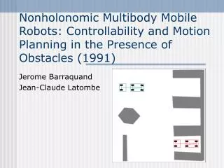
Nonholonomic Multibody Mobile Robots: Controllability and Motion Planning in the Presence of Obstacles (1991) Jerome Barraquand Jean-Claude Latombe
Controllability • A robot is controllable if for any q1 and q2: a free path between from q1 to q2 a feasible free path from q1 to q2 • A multi-body robot is controllable if it can take on at least 2 different steering angles, j1 andj2, on the interval [-p, p), and can move both forward and backward
Motivation • How do we actually generate a feasible path? • Other algorithms first generate a free path ignoring nonholonomic constraints, then convert to a topologically equivalent feasible path. • We would like to take our constraints into account as we plan our path
Algorithm Overview • Series of hinged bodies with wheels on flat ground, no slipping • Front wheels have 2 different steering angles, jmin and jmax, in the range of [-p, p) • Arbitrary obstacles • Searches for a path from qinit to any configuration within a neighborhood of qgoal • Asymptotically complete • Optimal in number of reversals • Exponential in number of bodies of the robot
Summary of How It Works • Searches a tree where each node is a feasible configuration • At each step, considers only the option of setting the steering angle to jmin or jmax, backing up or going forward • Successors of a node represent configurations where the car can be dt0 time later
Summary of How It Works • Expand the tree in an order that minimizes reversals • Tricks to prune the tree • Limit your search depth (H) • Avoid visiting identical configurations (R)
Generating Successors • Consider only a set of discrete values for v and j, specifically v=-1 or 1, j =jmin or jmax. • Integrate velocity equations defined by nonholonomic systems over dt0 to compute each new position dx/dt = v cos(j) cos(q) dy/dt = v cos(j) sin(q) Ldq/dt = v sin(j)
Growing the Tree • Maintain fringe nodes in heap • Select the fringe node along a path with the least number of reversals, tie goes to shortest path • Terminate this node if it collides with an obstacle or is in a previously visited configuration • Mark node’s configuration as visited • Test if node’s configuration is in the neighborhood of the goal • Add node’s successors to fringe • Bound maximum search depth (H)
Node Deletion • A node is deleted (i.e. we don’t need to expand it) if: • The path between this node and this node’s parent collides with an obstacle use a bitmap to represent workspace • Current configuration is in the neighborhood of a previously visited configuration • Store an array A composed of 2R(p+2) parallelepipeds which maps entire configuration space • R is user provided tuning parameter, p is the number of bodies in the robot • Need two separate arrays for going forward and in reverse
Completeness and Optimality • Algorithm achieves controllability if dt0 is set small enough, and R and H are set large enough • Since nodes along paths with minimum number of reversals are expanded first, algorithm is optimal in number of reversals (if dt0, R, and H are fine enough)
Picking Tuning Parameters • Three tuning parameters dt0, R, and H • If algorithm returns failure, you don’t know if there is no solution or if dt0, R, and H were not set properly • Small dt0 might be necessary; results in much larger tree • Values of dt0, R, and H are dependent on each other; setting the parameters in the order dt0, H, and R works well • Guess dt0 using prior knowledge of the workspace • Can use faster algorithm ignoring nonholonomic constraints to test if solution is possible, then keep refining dt0 until solution is found
Performance • Exponential in the size of the configuration space (number of bodies of the robot) • Exponential in R, so in practice should be exponential in 1/dt0 • Not very practical for robots with more than 2 bodies, but can solve some difficult problems in reasonable amounts of time
Performance (in 1991) Random Obstacles Car That Can Only Turn Left jmax=45o, jmin=22.5o, R=9, 20 sec. jmax=45o, R=9, 2 min.
Performance (in 1991) jmax=45o, R=7, 20 min.
Algorithm Evaluation • General/Extendable: With modest changes, could work for other types of robots with different nonholonomic constraints or in a 3D environment; room for speed optimizations dealing with the tree search • Complete and Optimal: In the asymptotic case will always find a path (if one exists) with the minimum number of reversals • Approximate: Final configuration is in the neighborhood of goal • Discrete Steering Angles: Does not take advantage of possibility of steering angles on continuous interval • Use more discrete steering angles than 2 (increases branching factor) • Use some kind of smoothing algorithm
Algorithm Evaluation (Cont) • Minimizes Reversals: Better than most algorithms but still not necessarily what you want; perhaps could try a different evaluation metric