Classification, Part 1
Classification, Part 1. BMTRY 726 4/8/14. Classification. Assuming we have data with 2 or more groups, we may want to determine which group an observation belongs too Thus the goal of classification analysis is to find a “good” rule to assign observations to an appropriate group…

Classification, Part 1
E N D
Presentation Transcript
Classification, Part 1 BMTRY 726 4/8/14
Classification Assuming we have data with 2 or more groups, we may want to determine which group an observation belongs too Thus the goal of classification analysis is to find a “good” rule to assign observations to an appropriate group… But how do we do that?
Decision Theory How does probability play a role in decision making? Example: we want determine if a patient has lung cancer or not based on a CT-scan. -inputs x: set of pixel intensities for our image -outcome y: lung cancer (Y/N) Consider probability of a subject’s class given their image using Bayes’ theorem Intuitively we choose the class with the higher posterior probability
Definitions in Classification We are looking for classification rules that minimize our total expected misclassification cost/loss
Minimizing Misclassification Rate A simple cost function is to minimize the number of observations we misclassify 1. Develop a rule that assigns classes to each observation 2. Rule divides feature space X into regions Rk (decision regions). Boundaries between these regions are called decision boundaries. 3. Calculate the probability of a misclassification. Consider a 2 class example, a mistake occurs when an input vector belonging to C1 is assigned to C2 The probability of a mistake is:
The minimum probability of making a mistake occurs if x assigned to class with the largest posterior probability Generalized to k classes, it is often easier to maximize the probability of being correct which is maximized when regions Rk chosen such that each x assigned to class with largest posterior probability
Minimizing Expected Loss Often, minimizing misclassification is too simplistic We may need to consider that some wrong decisions are worse than others -lung cancer: incorrectly diagnosing a cancer patient as healthy can lead to premature death! We can consider more formalized cost/loss functionswhich represent single measures of loss for each action Goal then becomes to minimize the total cost/loss In our cancer example consider a loss matrix:
The optimal solution minimizes the loss function Problem is the loss function depends on true class, which is unknown (for new observations) For a vector x, uncertainty on true class can be expressed as a joint probability We then minimize the expected loss w.r.t. this distribution Goal to choose regions Rj to minimize this expected loss- implies for each x assigned to class j should minimize
Reject Option Classification errors can also result from: -regions of input space where the largest posterior probabilities, , are small -posterior probabilities for 2 or more classes are similar It may be better to avoid making decisions for difficult cases in attempt to reduce error rate Referred to as rejection option- set specific region where classifier does not make a decision This does require there is some means (e.g. expert opinion) to make decision about those points within this region
Inference and Decision Classification problem can be broken into two stages -inference stage: use training data to learn a model for -decision stage: use estimated posterior probability to make optimal class assignment Alternatively we can solve both problems together an learn a function that maps inputs x directly into decisions Such a function is called a discriminant function (this is what we will address initially)
Approaches • Solve inference problem of finding posterior probabilities for each class Ck individually -use Bayes’ thm and find posterior class probabilities -use posteriors to make optimal decision -referred to as generative models (2) Solve inference problem by determining -use posteriors to make optimal decision -referred to as discriminative models (3) Find function f(x) (called a discriminant function) that maps each point x directly into class label -NOTE: in this case, probabilities play no role
Approaches There are merits and drawbacks to each of the approaches First approach most computationally demanding especially if x is large… However, only approach that estimates prior class probabilitesp(Ck) and marginal probablities on data p(x) If really only want to do classification, all this not necessary and only really need posterior probabilites provided in second approach Third approach even more simple (most computationally easy) but we now do not have estimates of posterior probabilities on the classes which may be desirable
Approaches We will initially focus on discriminant functions (approach 3 and on some level 2) We still want to minimize total expected cost In this case, our optimal classification rule classifies x0 to kth group if smallest among the groups Equivalently, for equal misclassification costs, classify x0 to k if is the largest- from Bayes we obtain the posterior probabilities for the kth class
Other Considerations So it seems like we have the information we need… However, we don’t know what the fk(x)’s are We must estimate these as well (and we will get to that) We also want to evaluate the performance of any classifier Apparent error rate: crosstabulate the actual class of observations in the training sample and the predicted classes for the same observations. Then count the number incorrectly classified.
Other Considerations Apparent error rate not of greatest interest though Much more interested in error on future observations since apparent error rate generally very optimistic due to overfitting To avoid overfitting we can use some strategies discussed earlier -Split data into test and training sets (in n large) -K-fold cross-validation -Generalized cross-validation -Bootstrap re-sampling To name a few…
Discriminant Functions Takes input vector x and assigns it to one of K classes (CK) -linear discriminantfunction means function is linear Simplest linear discriminant function: 1st consider 2 class case: -Input vector x assigned to class C1 if y(x)>0 and class C2 otherwise -Decision boundary defined by y(x)>0 -b0 determines boundary location
Linear Discriminant Functions In order to generalize this to K > 2 classes, we define one discriminant comprised of K linear functions: Decision boundary between j and k is a (D-1)-dimensional hyperplane defined by: Properties: -Singly connected -Convex
Least Squares Approach Assuming data contains K classes, we can create a matrix of K vectors of binary indicators Each class Ck has its own linear model Vector of weights for the kthmodel determined using least squares solution for vector describing the kthclass New input x assign to class for which is largest
Least Squares Approach In this setting we view the regression model as an estimate of a conditional expectation We can also think of this as an estimate of the posterior probability given our feature vector x Question: how good is this approximation -we can verify that -but there are some issues…
Least Squares Approach Positive aspects of this approach: -Closed for solution for discriminant function parameters -Familiarity in stats community Some obvious problems with this approach: -model output should represent probability but not constrained on (0,1) interval -Poor separation of classes if a region assigned only a small posterior probability -Lacks robustness to outliers (even worse for classification problems)
Outliers… Small “posterior probability”…
So far we have made no assumptions about the distribution of the data Decision theory suggests that we need to know the posterior class probability for optimal classification This brings us back to Bayes… We can see that having fk(x) can help us classify observations Many techniques are based on models for the class densities Linear (and quadratic) discriminant analysis assumes MVN
Linear Discriminant Analysis: 2 Class Case First assume our features are MVN with equal covariances Our fk(x)’s are: In normal theory, we often resort to a likelihood ratio test… what if we consider something like that here? The problem is we are interested in our posterior class probabilities rather than fk(x)…
2 Class Case Assume covariances are equal If the last quantity is <0, we classify an observation as belonging to class 1
2 Class Case Instead of the ration of f1(x) to f2(x) , consider the ratio of the conditional probabilities
2 Class Case We can think of this as the log odds of being in class 1 versus class 2 Therefore we make our decision about class assignment based on whether this ratio is larger or smaller than 0 Our decision boundary between the two classes occurs where This boundary represents a hyperplane in p dimensions (based on the p features defined in x)
Linear Discriminant Analysis We can generalize this to more than 2 classes The more general form of the linear discriminant function for LDA is: The decision boundary between classes is defined by multiple hyperplanes defined by each line where
LDA and Least Squares In the 2 class case there is a correspondence between our least squares classifier and LDA LDA classifies and observed x to class 2 if It can be shown that the coefficients vector from LS is proportional to the LDA direction shown above Decision rules only the same if N1 = N2 However for more than 2 classes, LDA and linear regression loose this correspondence
From a least squares standpoint, we can also think about classification via LDA as a dimensionality reduction problem For 2 class case, we use p inputs (vector x) and project into one direction represented by: Thresholding so that y > 0 classifies C1 same as least squares Problem is loss of information… what may have been well separated in p-dimensional space isn’t in 1-d space Instead adjust weights b to select a projection that maximizes separation
Quadratic Discriminant Analysis One very strong assumption we’ve sort of glossed over in LDA is the assumption that all covariance matrices are equal If this assumption does not hold, we can’t simplify our log ratio quite as easily The first term can’t be dropped…
Quadratic Discriminant Analysis We can simplify this a little bit… Our final discriminant function in this case becomes
Quadratic Discriminant Analysis Our discriminant function is no longer linear Hence we refer to this as quadratic discriminant analysis
General notes So how do we decide between linear and quadratic discriminant analysis? We need to check if our covariances for our two (or more) populations are the same -Bartlett’s test (as always, interpret with caution)