Machine Learning for Analyzing Brain Activity
Machine Learning for Analyzing Brain Activity. Tom M. Mitchell Machine Learning Department Carnegie Mellon University October 2006 Collaborators: Rebecca Hutchinson, Marcel Just, Mark Palatucci, Francisco Pereira, Rob Mason, Indra Rustandi, Svetlana Shinkareva, Wei Wang.


Machine Learning for Analyzing Brain Activity
E N D
Presentation Transcript
Machine Learning for Analyzing Brain Activity Tom M. Mitchell Machine Learning Department Carnegie Mellon University October 2006 Collaborators: Rebecca Hutchinson, Marcel Just, Mark Palatucci, Francisco Pereira, Rob Mason, Indra Rustandi, Svetlana Shinkareva, Wei Wang
improving performanceat some taskthrough experience Learning =
Learning to Predict Emergency C-Sections [Sims et al., 2000] 9714 patient records, each with 215 features
Learning to detect objects in images (Prof. H. Schneiderman) Example training images for each orientation
Learning to classify text documents Company home page vs Personal home page vs University home page vs …
Reinforcement Learning [Sutton and Barto 1981; Samuel 1957]
Mining Databases Object recognition Machine Learning - Practice Speech Recognition • Reinforcement learning • Supervised learning • Bayesian networks • Hidden Markov models • Unsupervised clustering • Explanation-based learning • .... Control learning Text analysis
Machine Learning - Theory • Similar theories for • Reinforcement skill learning • Unsupervised learning • Active student querying • … PAC Learning Theory (for supervised concept learning) # examples (m) representational complexity (H) error rate (e) • … also relating: • # of mistakes during learning • learner’s query strategy • convergence rate • asymptotic performance • … failure probability (d)
Brain scans can track activation with precision and sensitivity [from Walt Schneider]
ERP Time course with millisecond precision 10 ms = 10 % of human production cycle • DTI Connections tracing millimeter precision 1 mm connection ~10k fibers, or 0.0001% of neurons Human Brain Imaging • fMRI Location with millimeter precision 1 mm3 = 0.0004% of cortex [from Walt Schneider]
Can we train program to classify what you’re thinking about? “reading a word about tools” or “reading a word about buildings” ? Observed fMRI: … … time • Train classifiers of form: • fMRI(t, t+1,... t+d) CognitiveProcess • e.g., fMRI(t, t+1,... t+4) = {tools, buildings, fish, vegetables, ...}
Reading a noun (15 sec) [Rustandi et al., 2005]
Representing Meaning in the Brain Study brain activation associated with different semantic categories of words and pictures Categories: vegetables, tools, trees, fish, dwellings, building parts Some experiments use block stimulus design • Present sequence of 20 words from same category, classify the block of words Some experiments use single stimuli • Present single words/pictures for 3 sec, classify brain activity for single word/picture
Classifying the Semantic Category of Word Blocks Learn fMRI(t,...t+32) word-category(t,...t+32) • fMRI(t1...t2) = 104 voxels, mean activation of each during interval [t1 t2] Training methods: • train single-subject classifiers • Gaussian Naïve Bayes P(fMRI | word-category) • Nearest nbr with spatial-correlation as distance • SVM, Logistic regression, ... Feature selection: Select n voxels • Best accuracy: reduce 104 voxels to 102
Mean Activation per Voxel for Word Categories Classification accuracy 1.0 (tools vs dwellings) on each of 7 human subjects (trained on indiv. human subjects) Presentation 1 Presentation 2 Tools Dwellings one horizontal slice, from one subject, ventral temporal cortex [Pereira, et al 2004]
C F1 F2 … Fn • Gaussian Naïve Bayes (GNB) classifier* for <f1, … fn> C. Assume the fj are conditionally independent given C. • Training: • For each class value, ci, estimate • For each feature Fj estimate Normal distribution Classify new instance Use Bayes rule: *assumes feature values are conditionally independent given the class
Results predicting word block semantic category Mean pairwise prediction accuracy averaged over 8 subjects: Random guess: 0.5 expected accuracy Ventral temporal cortex classifiers averaged over 8 subjects: • Best pair: Dwellings vs. Tools (1.00 accuracy) • Worst pair: Tools vs. Fish (.40 accuracy) • Average over all pairs: .75 Averaged over all subjects, all pairs: • Full brain: .75 (individual subjects: .57 to .83) • Ventral temporal: .75 (individuals: .57 to .88) • Parietal: .70 (individuals: .62 to .77) • Frontal: .67 (individuals: .48 to .78)
Question: Are there consistently distinguishable and consistently confusable categories across subjects?
Six-Category Study: Pairwise Classification Errors (ventral temporal cortex) * Worst * Best
Question: Can we classify single, 3-second word presentation?
Classifying individual word presentations Accuracy of up to 80% for classifying whether word is about a “tool” or a “dwelling” Rank accuracy of up to 68% for classifying which of 14 individual words (6 presentations of each word) Category classification accuracy is above chance for all subjects. Individual word classification accuracy is not consistent across subjects
Question: Where in the brain is the activity that discriminates word category?
Learned Logistic Regression Weights: Tools (red) vs Buildings (blue)
Accuracy of searchlights: Bayes classifier Accuracy at each voxel with a radius 1 searchlight
Regions that encode ‘tools’ vs. ‘dwellings’ “searchlight” classifier at each voxel uses only the voxel and its immediate neighbors Accuracy at each significant searchlight [0.7-0.8] “tools” vs. “dwellings
The distinguishing voxels occur in sensible areas:dwellings activate parahippocampal place areatools activate motor and premotor areas
What is the relation between the neural representation of a word in two different languages in the brain of a bilingual? Tested 10 Portuguese-English bilinguals in English and in Portuguese, using the same words
Identifying categories (tool or dwelling) within languages for individual subjects • using naïve bayes classifier
Identifying categories across languages for individual subjects (rank accuracy) Across Languages
What is the relation between the neural representation of an object when it is referred to by a word versus when it is depicted by a line drawing?
Schematic representation of experimental design for (A) pictures and (B) words experiments
It is easier to identify the semantic category of a picture a subject is viewing than a word he/she is reading Pictures accuracy Words accuracy
Can a classifier be trained in one modality, and then accurately identify activation patterns in the other modality?
Cross-Modal identification accuracy is high, in both directions Word to picture Picture to word
Can a classifier be trained on a group of human subjects, then be successfully applied to a new person?
Picturecategory accuracy within and between subjects The classifiers work well across subjects; for “bad” subjects, the identification is even better across than within subjects Within subject accuracy Between subject accuracy
Locations of diagnostic voxels across subjectsTool voxels are shown in blue, dwellings voxels are shown in redL IPL indicated with a yellow circle;activates during imagined or actual grasping (Crafton et al., 1996) Subj 1 Subj 2 Subj 3 Subj 4 Subj 5
Voxel Locations are Similar for Pictures and Words Pictures Tools: L IPL L postcentral L middle temporal Cuneus Dwellings (positive weights): L/R Parahippocampal gyrus Cuneus Words Tools: L IPL L postcentral L precentral L middle temporal Dwellings (positive weights): L/R Parahippocampal gyrus Interpretation: L IPL – imaginary grasping (of tools, here) (Crafton et al., 1996) Parahippocampal gyrus – formation and retrieval of topographical memory; plays a role in perception of landmarks or scenes
Lessons Learned Yes, one can train machine learning classifiers to distinguish a variety of cognitive states/processes • Picture vs. Sentence • Ambiguous sentence vs. unambiguous • Nouns about “tools” vs. nouns about “dwellings” • Train on Portuguese words, test on English • Train on words, test on pictures • Train on some human subjects, test on others Failures too: • True vs. false sentences • Negative sentence (containing “not”) vs. affirmative ML methods: • Logistic regression, NNbr, Naïve Bayes, SVMs, LogReg, … • Feature selection matters: searchlights, contrast to fixation, ... • Case study in high dimensional, noisy classification [MLJ 2004]
[Science, 2001] [Machine Learning Journal, 2004] [Nature Neuroscience, 2006]
Input stimuli: ? Can we learn to classify/track multipleoverlapping processes (with unknown timing)? Read sentence View picture Decide whether consistent Observed fMRI: Observed button press:
Red to be learned sentence sentence Process: ReadSentence Duration d: 11 sec. P(Process = ReadSent) P(Offset times): Response signature W: Input Stimulus : picture Hidden Process Models Timing landmarks : ¢2 ¢ 1 ¢ 3 Process instance:4 Process h: ReadSentence Timing landmark : 3 Offset time O: 1 sec Start time´ + O Configuration C of Process Instances h1, 2, … i 1 4 2 3 Observed data Y:
Voxel v, time t The HPM Graphical Model Probabilistically generate data Yt,vusing a configuration of N process instances 1, ... n observed unobserved Stimulus(1) Stimulus(2) ProcessType(1) ProcessType(2) Offset(1) Offset(2) S S StartTime(1) StartTime(2) 2contribution to Yt,v 1contribution to Yt,v observed data Yt,v
Learning HPMs • Known process IDs,start times: • Least squares regression, eg. Dale[HBM,1999] • Ordinary least sq if assume noise indep over time • Generalized least sq if assume autocorrelated noise • Unknown start times: EM algorithm (Iteratively reweighted least squares) • Repeat: • E: estimate distribution over latent variables • M: choose parameters to maximize expected log full data likelihood Y = X h + ε
HPM: Synthetic Noise-Free Data Example Process 1: Process 2: Process 3: Process responses: Time ProcessID=1, S=1 Process instances: ProcessID=2, S=17 ProcessID=3, S=21 observed data
true signal Observed noisy signal true response W learned W Process 1 Process 2 Process 3 Figure 1. The learner was given 80 training examples with known start times for only the first two processes. It chooses the correct start time (26) for the third process, in addition to learning the HDRs for all three processes.
Inference with HPMs • Given an HPM and data set • Assign the Interpretation (process IDs and timings) that maximizes data likelihood • Classification = assigning the maximum likelihood process IDs y = X h + ε