Download

1 / 48
480 likes | 645 Vues
Part of Speech Tagging & Hidden Markov Models. Mitch Marcus CSE 391. NLP Task I – Determining Part of Speech Tags. The Problem:. NLP Task I – Determining Part of Speech Tags. The Old Solution: Depth First search.

E N D
Part of Speech Tagging& Hidden Markov Models Mitch Marcus CSE 391
NLP Task I – Determining Part of Speech Tags • The Problem:
NLP Task I – Determining Part of Speech Tags • The Old Solution: Depth First search. • If each of n words has k tags on average, try the nk combinations until one works. • Machine Learning Solutions: Automatically learn Part of Speech (POS) assignment. • The best techniques achieve 97+% accuracy per word on new materials, given large training corpora.
What is POS tagging good for? • Speech synthesis: • How to pronounce “lead”? • INsult inSULT • OBject obJECT • OVERflow overFLOW • DIScount disCOUNT • CONtent conTENT • Stemming for information retrieval • Knowing a word is a N tells you it gets plurals • Can search for “aardvarks” get “aardvark” • Parsing and speech recognition and etc • Possessive pronouns (my, your, her) followed by nouns • Personal pronouns (I, you, he) likely to be followed by verbs
Equivalent Problem in Bioinformatics • Durbin et al. Biological Sequence Analysis, Cambridge University Press. • Several applications, e.g. proteins • From primary structure ATCPLELLLD • Infer secondary structure HHHBBBBBC..
Simple Statistical Approaches: Idea 2 For a string of words W = w1w2w3…wn find the string of POS tags T = t1 t2 t3 …tn which maximizes P(T|W) • i.e., the most likely POS tag ti for each word wi given its surrounding context
The Sparse Data Problem … A Simple, Impossible Approach to Compute P(T|W): Count up instances of the string "heat oil in a large pot" in the training corpus, and pick the most common tag assignment to the string..
A BOTECEstimate of What We Can Estimate • What parameters can we estimate with a million words of hand tagged training data? • Assume a uniform distribution of 5000 words and 40 part of speech tags.. • Rich Models often require vast amounts of data • Good estimates of models with bad assumptions often outperform better models which are badly estimated
A Practical Statistical Tagger II But we can't accurately estimate more than tag bigrams or so… Again, we change to a model that we CAN estimate:
A Practical Statistical Tagger III So, for a given string W = w1w2w3…wn, the taggerneeds to find the string of tags T which maximizes
Training and Performance • To estimate the parameters of this model, given an annotated training corpus: • Because many of these counts are small, smoothing is necessary for best results… • Such taggers typically achieve about 95-96% correct tagging, for tag sets of 40-80 tags.
.3 .02 Adj Det .6 .47 .51 .1 Hidden Markov Models This model is an instance of a Hidden Markov Model. Viewed graphically: .3 Noun .7 Verb
.02 .3 .3 Det Adj Noun Verb .47 .6 .7 .51 .1 P(w|Det) P(w|Adj) P(w|Noun) a .4 good .02 price .001 the .4 low .04 deal .0001 Viewed as a generator, an HMM:
A Practical Statistical Tagger IV • Finding this maximum can be done using an exponential search through all strings for T. • However, there is a linear time solution using dynamic programming called Viterbi decoding.
Parameters of an HMM • States: A set of states S=s1,…,sn • Transition probabilities: A= a1,1,a1,2,…,an,nEach ai,jrepresents the probability of transitioning from state sito sj. • Emission probabilities: A set B of functions of the form bi(ot) which is the probability of observation otbeing emitted by si • Initial state distribution: is the probability that si is a start state
The Three Basic HMM Problems • Problem 1 (Evaluation): Given the observation sequence O=o1,…,oTand an HMM model , how do we compute the probability of O given the model? • Problem 2 (Decoding): Given the observation sequence O=o1,…,oTand an HMM model , how do we find the state sequence that best explains the observations? (This and following slides follow classic formulation by Rabiner and Juang, as adapted by Manning and Schutze. Slides adapted from Dorr.)
The Three Basic HMM Problems • Problem 3 (Learning): How do we adjust the model parameters , to maximize ?
Problem 1: Probability of an Observation Sequence • What is ? • The probability of a observation sequence is the sum of the probabilities of all possible state sequences in the HMM. • Naïve computation is very expensive. Given T observations and N states, there are NT possible state sequences. • Even small HMMs, e.g. T=10 and N=10, contain 10 billion different paths • Solution to this and problem 2 is to use dynamic programming
Forward Probabilities • What is the probability that, given an HMM , at time t the state is i and the partial observation o1 … ot has been generated?
Forward Algorithm • Initialization: • Induction: • Termination:
Forward Algorithm Complexity • Naïve approach takes O(2T*NT) computation • Forward algorithm using dynamic programming takes O(N2T) computations
Backward Probabilities • What is the probability that given an HMM and given the state at time t is i, the partial observation ot+1 … oTis generated? • Analogous to forward probability, just in the other direction
Backward Algorithm • Initialization: • Induction: • Termination:
Problem 2: Decoding • The Forward algorithm gives the sum of all paths through an HMM efficiently. • Here, we want to find the highest probability path. • We want to find the state sequence Q=q1…qT, such that
Viterbi Algorithm • Similar to computing the forward probabilities, but instead of summing over transitions from incoming states, compute the maximum • Forward: • Viterbi Recursion:
Viterbi Algorithm • Initialization: • Induction: • Termination: • Read out path:
Problem 3: Learning • Up to now we’ve assumed that we know the underlying model • Often these parameters are estimated on annotated training data, but: • Annotation is often difficult and/or expensive • Training data is different from the current data • We want to maximize the parameters with respect to the current data, i.e., we’re looking for a model , such that
Problem 3: Learning (If Time Allows…) • Unfortunately, there is no known way to analytically find a global maximum, i.e., a model , such that • But it is possible to find a local maximum • Given an initial model , we can always find a model , such that
Forward-Backward (Baum-Welch) algorithm • Key Idea: parameter re-estimation by hill-climbing • From an arbitrary initial parameter instantiation , the FB algorithm iteratively re-estimates the parameters, improving the probability that a given observation was generated by
Parameter Re-estimation • Three parameters need to be re-estimated: • Initial state distribution: • Transition probabilities: ai,j • Emission probabilities: bi(ot)
Re-estimating Transition Probabilities • What’s the probability of being in state si at time t and going to state sj, given the current model and parameters?
Re-estimatingTransition Probabilities • The intuition behind the re-estimation equation for transition probabilities is • Formally:
Re-estimatingTransition Probabilities • Defining As the probability of being in state si, given the complete observation O • We can say:
Re-estimating Initial State Probabilities • Initial state distribution: is the probability that si is a start state • Re-estimation is easy: • Formally:
Re-estimation of Emission Probabilities • Emission probabilities are re-estimated as • Formally:where • Note that here is the Kronecker delta function and is not related to the in the discussion of the Viterbi algorithm!!
The Updated Model • Coming from we get to by the following update rules:
Expectation Maximization • The forward-backward algorithm is an instance of the more general EM algorithm • The E Step: Compute the forward and backward probabilities for a give model • The M Step: Re-estimate the model parameters