Download
1 / 24
240 likes | 398 Vues
Photometric Monitoring of the Field of Open Star Cluster M23. Jeff Wilkerson Iowa Academy of Science April 21, 2012. Sensitive to Variability on a Wide Range of Timescales: I. Tenths of seconds to seconds Occultation and microlensing events Brief flares

E N D
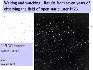
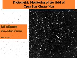
Photometric Monitoring of the Field of Open Star Cluster M23 Jeff Wilkerson Iowa Academy of Science April 21, 2012
Sensitive to Variability on a Wide Range of Timescales: • I. Tenths of seconds to seconds • Occultation and microlensing events • Brief flares • II. Tenths of hours to a few days • Flares in long period variables • Delta Scuti stars • Traditional flare stars • Eclipsing binaries • Transiting planets III. Days to hundreds of days • Long period pulsating variable stars • Eclipsing binary stars • Cataclysmic variable stars • Cepheid variables • Period-to-period variability in long period variables • Rotating variable stars in young clusters IV. Years to decades • Luminosity stability • Solar-like cycles • Period-to-period variability in long period variables • Proper motions of stars Have observed 61“classical” variable stars to date, 59 of them newly discovered
Student Participation: Zebadiah Howes Buena Vista Univ. Travis DeJong Dordt College Forrest Bishop Decorah High School Ujjwal Joshi Nathan Rengstorf Andrea Schiefelbein Todd Brown Brajesh Lacoul Kari Frank Alex Nugent Drew Doescher Alex Sperry Jennifer Schulz Clara Olson Robyn Siedschlag Siri Thompson Matt Fitzgerald Heather Lehmann Amalia Anderson Hilary Teslow Steve Dignan Kirsten Strandjord Donald Lee-Brown Andrew Becklin Support: Roy J. Carver Charitable Trust (Grant #00-50) Luther College R.J. McElroy Trust/Iowa College Foundation American Astronomical Society
Short (II) Timescales: (tenths of hours to a few days) • Primarily two types of objects here: • Flare stars • Eclipsing binaries From Contemporary Activities in Astronomy, by Hoff and Wilkerson
How do we find these? WSVI-statistic test • Fit a second-order polynomial to signalas a function of normalization factor • Define the WSVI* statistic to measure the deviation of a star’s signal from the polynomial fit using paired observations • Find the mean WSVI for a subset of stars • Measure each star’s WSVI deviation from the mean of its subset * Based on a variability index developed by Welch and Stetson (AJ, 105, 1993)
Eclipsing Binaries Period = 0.32866 days Period = 0.5455059(2) days Period = 0.20730 days Period = 5.5 days Period = 1.883360(2) days Period = 9.48665 days
<T2-T1>odd = 0.710±.053 hr <T2-T1>even = 0.782±.045 hr <T3-T2>odd = 0.683±.042 hr <T3-T2>even = 0.703±.068 hr <T4-T3>odd = 0.865±.041 hr <T4-T3>even = 0.785±.075 hr 3s limit on LoS eccentricity ≈ 0.007 P = 1.883360(2)d mO-C, even = 0.00024±.0009d(unc. ≈ 0.2 sec.)mO-C, odd = -0.00025±.0009d 3s limit on any variations ≈ 0.012d 3s limit on projection of eccentricity ≈ 0.001 In general: (dP/dt)/P = 2(dm/dt)/(m1+m2) + 3(dm1/dt)(m1-m2)/m1m2 + 3K For us, 3s limit on dP/dt comes from 3s limit on O-C in 2011 vs. 2005 of 0.012d Pavg – Pobs = 5.2x10⁻⁶d DP = 1.04x10⁻⁵d in 2200 days (dP/dt)max = 4.5x10⁻⁹ Use sizes from eclipse timing and color to estimate m1 = 0.7Mʘ and m2 = 0.3Mʘ. dm1/dt < [(0.7Mʘ)(0.3Mʘ)/3Mʘ](4.5x10-9)/1.88d = 6x10⁻⁸Mʘ/year
sodd = 71.3 ADU seven = 206.6 ADU If the standard deviations are distributed normally then the variance of the of the standard deviation is: Var(s) = 1/N[N-1-2G2(N/2)/G2((N-1)/2)]Ns2/(N-1) Yields one standard deviation uncertainties: sodd = 71.3 +/-12.9ADU seven = 206.6+/-33.3 ADU (Ta/Tb)4 = Depth1/Depth2
One last check for a third star <T2-T1> = 0.746±.035 hr <T4-T3> = 0.825±.042 hr <T4-T2> = 1.494±.038 hr <T3-T1> = 1.437±.037 hr About 40% of the light goes away in either primary or secondary eclipse Total Light = C’(d12 +d22) = C[(.786)2 + (1.466)2] = C(.618 + 2.149) = C2.77 Eclipse timing actually gives minimum large object radius due to orbital inclination. Fraction of total area from smaller object= 0.618/2.77 = 0.22 What if the secondary object is dark? B-V = 1.415; V = 15.55 Assume reddening of cluster, = .356; (B-V)0= 1.059 Rstar≈0.80Rʘ Now need (Rdark/Rstar)2=0.40 Rdark≈0.80Rstar≈0.50Rʘ But we know brown dwarf stars have R ≈0.10Rʘ Assuming Rstar actually 2s below mean measured value and Rdark 2s above mean measured value yields fractional areal coverage of 0.355. If actual eclipse depth is 2s below mean measured value it would be 0.381.
Long (IV) Timescales: a variance test We claim stars with F-Stat > 4.70 are intrinsically variable High cutoff chosen so <FAP> ~0 Removed 7 stars with artificially high F-Stats: - 6 due to close neighbor interference - 1 due to transiting asteroid stars with F-Stat > 4.70 are variable +20 stars → 55 remaining stars with F-Stat>4.70
Pulsating Variables in the M23 Field Properties: Period: DCDFT Color: R-I Amplitude: 4-96% Asymmetry: Risetime/Period Mean Magnitude: (96+4)/2
Populations of Pulsating Stars We see many more lower A stars than higher A stars. Recognize that detection efficiency is lower for lower A stars as well. Fit a power law; extrapolate to threshold; use scatter to determine detection efficiency as a function of both magnitude and amplitude. Estimate the percentage of stars with A>0.22 mag. and P>10 days as : 3.6±0.6%. With cluster members removed the number is: 7.2±1.2%.
Interesting Stars: The Yellow Stars A likely RV Tau variable A likely Cepheid variable
Define Short-term Photometric Resolution (STPR) as s/m for a Gaussian fit to a histogram of several hundred signal measurements for a given star and Long-term Photometric Resolution (LTPR) as s/m for the nightly average signal measure of a given star over an entire campaign. At large signal values STPR approaches a constant (plateau) value determined by our frame normalization, itself limited by scintillation. For faint stars STPR increases as signal-1. In between STPR increases as signal-1/2. Counting statistics of the stellar signal measurement dominate STPR in this region. Functional fits shown of form: STPR=[(C1)² + (C2signal-1/2)² + (C3signal)2]1/2
Star 16 Star 41 Star 69 Star 166 Star 519 Star 1267
CONCLUSION • We have a unique data set that offers unprecedented temporal coverage of >1600 stars down to 19th magnitude, yielding a detection of variability in about 8% of the field stars. • Have measured eclipsing binary periods down to tenths or hundredths of a second. Variation in orbital parameters gives information on perturbations in the system. Expect detections or stringent upper limits to appear in the next few years. • Strong evidence of two classes of pulsating stars (high and low amplitude) with different pulsation behavior • Distinct classes of pulsational behavior have emerged. Any model or models of these stars must account for the observed intra-group and inter-group homogeneity and heterogeneity. • Brief, rare events in these stars and others are still being sought.