Download
1 / 25
250 likes | 384 Vues
Photometric Monitoring of the Field of Open Star Cluster M23. Jeff Wilkerson Luther College Iowa Academy of Science April 21, 2012. What We Do. Image M23 field every clear night every year and occasional other fields. From http://rst.gsfc.nasa.gov/Sect20/sun_mw+.jpg.

E N D
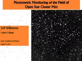
Photometric Monitoring of the Field of Open Star Cluster M23 Jeff Wilkerson Luther College Iowa Academy of Science April 21, 2012
What We Do Image M23 field every clear night every year and occasional other fields From http://rst.gsfc.nasa.gov/Sect20/sun_mw+.jpg Image durations: 2 to 12 seconds, unfiltered; use individually or summed FOV: ~1/2○ square M23 campaign durations: Late February to early October >1600 stars appear consistently in M23 field BVRI photometry occasionally for color correction to magnitude conversion and knowledge of variable star colors Equipment: 12” Meade Schmidt-Cassegrain; Apogee AP6E or SBIG STL-1001E camera Result: tens of thousands of images per field per year
Why Do We Do This? Because we can! http://www.hawaiimagazine.com/images/content/Mauna_Kea_wins_biggest_telescope/thirtymetertelescope.jpg
Sensitive to Variability on a Wide Range of Timescales: • I. Tenths of seconds to seconds • Occultation and microlensing events • Brief flares • II. Tenths of hours to a few days • Flares in long period variables • Delta Scuti stars • Traditional flare stars • Eclipsing binaries • Transiting planets III. Days to hundreds of days • Long period pulsating variable stars • Eclipsing binary stars • Cataclysmic variable stars • Cepheid variables • Period-to-period variability in long period variables • Rotating variable stars in young clusters IV. Years to decades • Luminosity stability • Solar-like cycles • Period-to-period variability in long period variables
Student Participation: Zebadiah Howes Buena Vista Univ. Travis DeJong Dordt College Forrest Bishop Decorah High School Ujjwal Joshi Nathan Rengstorf Andrea Schiefelbein Todd Brown Brajesh Lacoul Kari Frank Alex Nugent Drew Doescher Alex Sperry Jennifer Schulz Clara Olson Robyn Siedschlag Siri Thompson Matt Fitzgerald Heather Lehmann Amalia Anderson Hilary Teslow Steve Dignan Kirsten Strandjord Donald Lee-Brown Andrew Becklin Support: Roy J. Carver Charitable Trust (Grant #00-50) Luther College R.J. McElroy Trust/Iowa College Foundation American Astronomical Society
DATA PROCESSING • CALIBRATION • Dark Noise Correction • Flat Fielding • ALIGNMENT • Use a single frame forentire data set • STAR ID & EXTRACTION • Aperture photometry for signal determination • 256 Background regions • INTRA-NIGHT NORMALIZATION • INTER-NIGHT NORMALIZATION • MAGNITUDE CONVERSION • Frame Normalization • Identify four reference images from throughout the night • Calculate average flux for each star in all four frames – this is the reference signal • Determine the signal of each star in the frame to be normalized – this is the sample signal • Calculate (ref. signal/sample signal) for each star • Normalization factor = median of all ratios in (4)
Define Short-term Photometric Resolution (STPR) as s/m for a Gaussian fit to a histogram of several hundred signal measurements for a given star and Long-term Photometric Resolution (LTPR) as s/m for the nightly average signal measure of a given star over an entire campaign. At large signal values STPR approaches a constant (plateau) value determined by our frame normalization, itself limited by scintillation. For faint stars STPR increases as signal-1. In between STPR increases as signal-1/2. Counting statistics of the stellar signal measurement dominate STPR in this region. Functional fits shown of form: STPR=[(C1)² + (C2signal-1/2)² + (C3signal)2]1/2
Use Web Version of the BDAcatalog for magnitudes (Mermilliod and Paunzen , http://www.univie.ac.at/webda//). Find an empirical color equation for the system and apply it.
Short (II) Timescales: (tenths of hours to a few days) • Primarily two types of objects here: • Flare stars • Eclipsing binaries From Contemporary Activities in Astronomy, by Hoff and Wilkerson
How do we find these? WSVI-statistic test • Fit a second-order polynomial to flux as a function of normalization factor • Define the WSVI* statistic to measure the deviation of a star’s flux from the polynomial fit using paired observations • Find the mean WSVI for a subset of stars • Measure each star’s WSVI deviation from the mean of its subset * Based on a variability index developed by Welch and Stetson (AJ, 105, 1993)
Eclipsing Binaries Period = 0.32866 days Period = 0.54550 days Period = 0.20730 days Period = 5.5 days Period = 0.91475 days
Period Analysis All 4 of our short-period EBs show O-C variations consistent with cyclic. Kim et al. found that ~50% of EBs in the Mt. Suhora catalog show detectable variation in the their O-C diagrams; half of those were cyclic variations1,5. Could be light-time effect from the orbit of a third body. Only expect ~10-20% of systems to be triple2,4 but might expect much greater for short-period EBs since Kozai cycle is only known way to produce them3,4. Our apparent periods are short relative to most previously observed5. • Kim, C.-H., et al. 2003, in Stellar Astrophysics – a Tribute to Helmut A. Abt, Cheng, K.S., et al. (eds.), Kluwer Academic Publishers, 127-130. • Abt, H.A. 1983, Ann Rev A&A, 21, 343. • Kozai, Y. 1962, AJ, 67, 591. • Eggleton, P.P. and Kisseleva-Eggleton, L. 2006, Astrophys Space Sci, 304, 73. • Kreiner, J. M., et al. 2001, An Atlas of O-C Diagrams of Eclipsing Binary Stars, Parts 1-6, Cracow: Pedagogical University Press.
Long (IV) Timescales: An F-statistic test To get F-Stat: Take ratio of consecutive night variance to full data set variance. Histogram these values in 100 star chunks; fit a Gaussian measure each star’s deviation from the mean in standard deviations. F-Stat– Standard deviations from mean of set 50 stars with standard deviations greater than 5.5 F-Stat > 5.5
Pulsating Variables in the M23 Field Properties: Period: DCDFT Color: R-I Amplitude: 4-96% Asymmetry: Risetime/Period Mean Magnitude: (96+4)/2
Populations of Pulsating Stars We see many more lower A stars than higher A stars. Recognize that detection efficiency is lower for lower A stars as well. Fit a power lower; extrapolate to threshold; use scatter to determine detection efficiency as a function of both magnitude and amplitude. Estimate the percentage of stars with A>0.22 mag. and P>10 days as : 5.2±2.1%. With cluster members removed the number is: 10.4±4.2%.
Interesting Stars: The Yellow Stars A likely RV Tau variable A likely Cepheid variable
CONCLUSION • We have a unique data set that offer unprecedented temporal coverage of >1600 stars down to 19th magnitude. • Estimate ≥ or ≈ 10% of field stars in the direction of the center of the Galaxy are variable, probably largely from the galactic bulge. • Strong evidence of two classes of stars (high and low amplitude) with different pulsation behavior • A few interesting individual stars might help us understand these systems better. • Groups of stars with interesting behavior can lead to a better understanding of how these systems work as stability of pulsations over years or decades. • Eclipsing binaries appear to have shorter period cyclic behavior than typical – a clue to their formation?