Applications in Transportation Problems
Applications in Transportation Problems. Transportation Simplex Method: A Special-Purpose Solution Procedure. Transportation Simplex Method.

Applications in Transportation Problems
E N D
Presentation Transcript
Applications in Transportation Problems • Transportation Simplex Method: A Special-Purpose Solution Procedure
Transportation Simplex Method • To solve the transportation problem by its special purpose algorithm, the sum of the supplies at the origins must equal the sum of the demands at the destinations. • If the total supply is greater than the total demand, a dummy destination is added with demand equal to the excess supply, and shipping costs from all origins are zero. • Similarly, if total supply is less than total demand, a dummy origin is added. • When solving a transportation problem by its special purpose algorithm, unacceptable shipping routes are given a cost of +M (a large number).
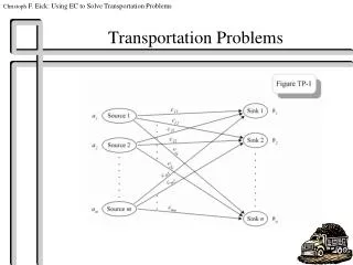
Transportation Simplex Method • A transportation tableau is given below. Each cell represents a shipping route (which is an arc on the network and a decision variable in the LP formulation), and the unit shipping costs are given in an upper right hand box in the cell. D1 D2 D3 Supply 30 20 15 S1 50 30 40 35 S2 30 Demand 25 45 10
Transportation Simplex Method • The transportation problem is solved in two phases: • Phase I -- Finding an initial feasible solution • Phase II – Iterating to the optimal solution • In Phase I, the Minimum-Cost Method can be used to establish an initial basic feasible solution without doing numerous iterations of the simplex method. • In Phase II, the Stepping Stone Method, using the MODI method for evaluating the reduced costs may be used to move from the initial feasible solution to the optimal one.
Transportation Simplex Method • Phase I - Minimum-Cost Method • Step 1:Select the cell with the least cost. Assign to this cell the minimum of its remaining row supply or remaining column demand. • Step 2:Decrease the row and column availabilities by this amount and remove from consideration all other cells in the row or column with zero availability/demand. (If both are simultaneously reduced to 0, assign an allocation of 0 to any other unoccupied cell in the row or column before deleting both.) GO TO STEP 1.
Transportation Simplex Method • Phase II - Stepping Stone Method • Step 1:For each unoccupied cell, calculate the reduced cost by the MODI method described below. Select the unoccupied cell with the most negative reduced cost. (For maximization problems select the unoccupied cell with the largest reduced cost.) If none, STOP. • Step 2:For this unoccupied cell generate a stepping stone path by forming a closed loop with this cell and occupied cells by drawing connecting alternating horizontal and vertical lines between them. Determine the minimum allocation where a subtraction is to be made along this path.
Transportation Simplex Method • Phase II - Stepping Stone Method (continued) • Step 3:Add this allocation to all cells where additions are to be made, and subtract this allocation to all cells where subtractions are to be made along the stepping stone path. (Note: An occupied cell on the stepping stone path now becomes 0 (unoccupied). If more than one cell becomes 0, make only one unoccupied; make the others occupied with 0's.) GO TO STEP 1.
Transportation Simplex Method • MODI Method (for obtaining reduced costs) Associate a number, ui, with each row and vj with each column. • Step 1:Set u1 = 0. • Step 2:Calculate the remaining ui's and vj's by solving the relationship cij = ui + vj for occupied cells. • Step 3:For unoccupied cells (i,j), the reduced cost = cij - ui - vj.
Example: Acme Block Co. (ABC) Acme Block Company has orders for 80 tons of concrete blocks at three suburban locations as follows: Northwood -- 25 tons, Westwood -- 45 tons, and Eastwood -- 10 tons. Acme has two plants, each of which can produce 50 tons per week. Delivery cost per ton from each plant to each suburban location is shown on the next slide. How should end of week shipments be made to fill the above orders? Acme
Example: ABC • Delivery Cost Per Ton NorthwoodWestwoodEastwood Plant 1 24 30 40 Plant 2 30 40 42
Example: ABC • Initial Transportation Tableau Since total supply = 100 and total demand = 80, a dummy destination is created with demand of 20 and 0 unit costs. Westwood Dummy Northwood Eastwood Supply 30 40 0 24 Plant 1 50 30 40 42 0 Plant 2 50 Demand 25 45 10 20
Example: ABC • Least Cost Starting Procedure • Iteration 1:Tie for least cost (0), arbitrarily select x14. Allocate 20. Reduce s1 by 20 to 30 and delete the Dummy column. • Iteration 2:Of the remaining cells the least cost is 24 for x11. Allocate 25. Reduce s1 by 25 to 5 and eliminate the Northwood column. continued
Example: ABC • Least Cost Starting Procedure (continued) • Iteration 3:Of the remaining cells the least cost is 30 for x12. Allocate 5. Reduce the Westwood column to 40 and eliminate the Plant 1 row. • Iteration 4:Since there is only one row with two cells left, make the final allocations of 40 and 10 to x22 and x23, respectively.
Example: ABC • Iteration 1 • MODI Method 1. Set u1 = 0 2. Since u1 + vj = c1j for occupied cells in row 1, then v1 = 24, v2 = 30, v4 = 0. 3. Since ui + v2 = ci2 for occupied cells in column 2, then u2 + 30 = 40, hence u2 = 10. 4. Since u2 + vj = c2j for occupied cells in row 2, then 10 + v3 = 42, hence v3 = 32.
Example: ABC • Iteration 1 • MODI Method (continued) Calculate the reduced costs (circled numbers on the next slide) by cij - ui + vj. Unoccupied CellReduced Cost (1,3) 40 - 0 - 32 = 8 (2,1) 30 - 24 -10 = -4 (2,4) 0 - 10 - 0 = -10
Example: ABC • Iteration 1 Tableau Westwood Dummy ui Northwood Eastwood 24 25 5 30 +8 40 20 0 Plant 1 0 -4 30 40 40 10 42 -10 0 Plant 2 10 vj 24 30 32 0
Example: ABC • Iteration 1 • Stepping Stone Method The stepping stone path for cell (2,4) is (2,4), (1,4), (1,2), (2,2). The allocations in the subtraction cells are 20 and 40, respectively. The minimum is 20, and hence reallocate 20 along this path. Thus for the next tableau: x24 = 0 + 20 = 20 (0 is its current allocation) x14 = 20 - 20 = 0 (blank for the next tableau) x12 = 5 + 20 = 25 x22 = 40 - 20 = 20 The other occupied cells remain the same.
Example: ABC • Iteration 2 • MODI Method The reduced costs are found by calculating the ui's and vj's for this tableau. 1. Set u1 = 0. 2. Since u1 + vj = cij for occupied cells in row 1, then v1 = 24, v2 = 30. 3. Since ui + v2 = ci2 for occupied cells in column 2, then u2 + 30 = 40, or u2 = 10. 4. Since u2 + vj = c2j for occupied cells in row 2, then 10 + v3 = 42 or v3 = 32; and, 10 + v4 = 0 or v4 = -10.
Example: ABC • Iteration 2 • MODI Method (continued) Calculate the reduced costs (circled numbers on the next slide) by cij- ui + vj. Unoccupied CellReduced Cost (1,3) 40 - 0 - 32 = 8 (1,4) 0 - 0 - (-10) = 10 (2,1) 30 - 10 - 24 = -4
Example: ABC • Iteration 2 Tableau Westwood Dummy ui Northwood Eastwood 25 25 30 +8 40 +10 0 24 Plant 1 0 -4 30 20 40 10 42 20 0 Plant 2 10 vj 24 30 36 -6
Example: ABC • Iteration 2 • Stepping Stone Method The most negative reduced cost is = -4 determined by x21. The stepping stone path for this cell is (2,1),(1,1),(1,2),(2,2). The allocations in the subtraction cells are 25 and 20 respectively. Thus the new solution is obtained by reallocating 20 on the stepping stone path. Thus for the next tableau: x21 = 0 + 20 = 20 (0 is its current allocation) x11 = 25 - 20 = 5 x12 = 25 + 20 = 45 x22 = 20 - 20 = 0 (blank for the next tableau) The other occupied cells remain the same.
Example: ABC • Iteration 3 • MODI Method The reduced costs are found by calculating the ui's and vj's for this tableau. 1. Set u1 = 0 2. Since u1 + vj = c1j for occupied cells in row 1, then v1 = 24 and v2 = 30. 3. Since ui + v1 = ci1 for occupied cells in column 2, then u2 + 24 = 30 or u2 = 6. 4. Since u2 + vj = c2j for occupied cells in row 2, then 6 + v3 = 42 or v3 = 36, and 6 + v4 = 0 or v4 = -6.
Example: ABC • Iteration 3 • MODI Method (continued) Calculate the reduced costs (circled numbers on the next slide) by cij - ui + vj. Unoccupied CellReduced Cost (1,3) 40 - 0 - 36 = 4 (1,4) 0 - 0 - (-6) = 6 (2,2) 40 - 6 - 30 = 4
Example: ABC • Iteration 3 Tableau Since all the reduced costs are non-negative, this is the optimal tableau. Westwood Dummy ui Northwood Eastwood 5 45 30 +4 40 +6 0 24 Plant 1 0 20 30 +4 40 10 42 20 0 Plant 2 6 vj 24 30 36 -6
Example: ABC • Optimal Solution FromToAmountCost Plant 1 Northwood 5 120 Plant 1 Westwood 45 1,350 Plant 2 Northwood 20 600 Plant 2 Eastwood 10 420 Total Cost = $2,490