Initialization of Numerical Models
280 likes | 377 Vues
Explore the evolution of CMEs using remote solar observations and numerical simulations. Discover how the CME Cone Model helps in fitting and predicting CME behavior. Learn about key parameters and interactions at Earth. Improve validation with multi-point observations.

Initialization of Numerical Models
E N D
Presentation Transcript
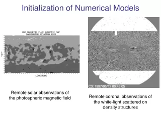
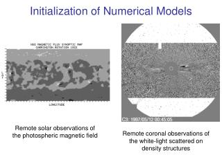
Initialization of Numerical Models Remote solar observations of the photospheric magnetic field Remote coronal observations of the white-light scattered on density structures
Observational evidence: • CME expands self-similarly • Angular extent is constant • Conceptual model: • CME as a shell-like region of enhanced density CME Cone Model [ Howard et al, 1982; Fisher & Munro, 1984 ] • Fitting of halo CMEs: • Various authors [Zhao, Liu, Michalek, Xie, etc] • Weak and fuzzy images • Cannot see “beyond” • STEREO will significantly improve accuracy
12 May 1997 1 May 1998 Application of the CME Cone Model 21 April 2002 24 August 2002 The heliospheric simulations may provide a global context of transient disturbances within a co-rotating, structured solar wind and they can serve as an intermediate solution until more sophisticated CME models become available.
Evolution of Parameters at Earth – Case A Poorly defined shock and its stand-off distance from the ejecta
Evolution of Parameters at Earth – Case B Accurate locations of stream boundaries and their rapid displacements are important for ICME properties at Earth
[ SAIC maps -- Pete Riley ] Effect of Fast-Stream Evolution Case A Case B Earth : Interaction region followed by shock and CME (not observed) Earth : Shock and CME (observed but shock front is radial)
[ WSA maps – Nick Arge ] Effect of Fast-Stream Evolution Case A Case B Earth : Interaction region followed by shock and CME (not observed) Earth : Shock and CME (observed but shock front is radial)
CMEs Cone Model Parameters CMEs fitted by:Liu (2005),Michalek (2003) and linear POS fit(CME list)
Magnetic Cloud and Fast Stream Post-Eruptive Flow MC Fast Stream Sudden Stream Displacement MC Fast Stream
Increasing Accuracy of Cone Model Specification STEREO-A ICME SUN EARTH STEREO-B
Geometric Localization of STEREO CMEs [ Pizzo and Biesecker, 2005 ]
Improving Validation of Cone Models – A Multi-point in-situ observations
Improving Validation of Cone Models – B Multi-point in-situ observations
May 12, 1997 Halo CME Running difference images fitted by the cone model
Case A Case B [ SAIC maps -- Pete Riley ] Fast-Stream Evolution Ambient state before the CME launch Disturbed state during the CME launch Ambient state after the CME launch
Cone Model Features Cone models – Intermediate solution until more realistic coronal models will enable routine application
Specification of Parameters Too many free parameters – while observed events may be reconstructed from case to case, their initialization cannot be automatized
Observed Ejecta Signatures and Shock Stand-off Interval Various interpretations of single-point, in-situ observations
WSA Model MAS Model UCSD Model Driving Heliospheric Computations at CCMC WSA Data MAS Data MAS Data UCSD Data In-Situ Data wsa2bc mas2bc mas2bc ucsd2bc coho2bc a3d2bc bnd.nc bnd.nc bnd.nc bnd.nc bnd.nc bnd.nc bnd.nc cone2bc ENLIL • Currently, there are three models (yellow) that can be used to drive ENLIL (green) • Computational system shares data sets (grey) and uses couplers (blue)
3-D Values at Time Level – tim.****.nc • Values are shown at Earth position (thick black line) and nearby grid points (light blue lines). • Observations from NASA-OMNIweb are shown by red dots. • Viewing evolution at nearby points can reveal effect of numerical resolution and can provide inclination of structures for geospace models • Values are shown on various slices passing through Earth • Current sheet is shown by white line • Planet positions are shown by black spheres • Calendar data and physical time correspond to file record number (****)