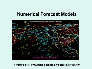
Numerical Forecast Models
Numerical Forecast Models. For more info: www.meted.ucar.edu/nwp/pcu1/ic2/index.htm. The Models. WRF (currently the NAM) US model output is at NCEP or NCAR-RAP GFS (NCEP) RUC (NCEP) ECMWF (Europe) www.ecmwf.int/ NoGaps (Navy) www.nwmangum.com/NOGAPS.phtml

Numerical Forecast Models
E N D
Presentation Transcript
Numerical Forecast Models For more info: www.meted.ucar.edu/nwp/pcu1/ic2/index.htm
The Models WRF (currently the NAM)US model output is at NCEP or NCAR-RAP GFS (NCEP) RUC (NCEP) ECMWF (Europe) www.ecmwf.int/ NoGaps (Navy) www.nwmangum.com/NOGAPS.phtml MM5 www.mmm.ucar.edu/mm5/mm5-home.html GEM (Canada) www.weatheroffice.gc.ca/model_forecast/index_e.html Eta(formerly the NAM) Many more – individuals, universities, and government agencies have their own! You too can write a model.
Did Lorenz (famous theoretical meteorologist) really say that?
You only have observations at specific places (stations) Convert derivatives to finite differences
So, models work by approximating the equations using finite differences on a model “grid.” (exception: spectral models) ∆x is the grid interval in the west-east direction. ∆y is south-north. ∆t is time.
The NAM-WRF, sometimes called the NMM (Non-hydrostatic Mesoscale Model) has a new staggered grid and a 12-km resolution.
You solve the finite difference equations for the points on a map. Depending on your computer size, you may only get a limited number of grid points. The limited area where your model is defined is called the “Domain”
The WRF model which is the basis for the North American Mesoscale model has a domain centered on - guess which continent. (March 2008)
If your domain is not global, you have artificial “boundaries”. Since these don’t exist in the real atmosphere, any effects from these boundaries are computational. The effects propagate into the interior as fast as air parcels move.
Once you define a domain, you need boundary conditions. The real Earth has topography. Your lower boundary must have mountains! 32-km Eta model terrain
Here’s a closer look at the Southwest and Northeast U.S. terrain in the 22 km Eta (22 km horizontal grid spacing). What do you think? (Remember the butterfly!)
13km RUC Terrain elevation - 100 m interval • Improvements expected from 13km RUC • Improved near-surface forecasts • Improved precipitation forecasts • Better cloud/icing depiction • Improved frontal/turbulence forecasts
Atmospheric models are three dimensional. You also need a vertical grid. Resolution in the vertical is much better than in the horizontal. But is it good enough?
The NAM-WRF has 60 vertical layers, as did the NAM-Eta. The top level in the NAM-WRF is 2 mb instead of the 25 mb Eta top level.
The NAM-WRF uses a vertical coordinate that is proportional to the surface pressure. So elevated terrain has very thin layers near the ground no matter how high it is. The old Eta had thin layers only near 1000 mb leading to errors in the western U.S. The vertical resolution is lowest near 500 mb and increases again near 250 mb for better depiction of jet stream shears.
Models have top and bottom boundaries. The real atmosphere doesn’t so how you program these affects model performance. Many models use nondimensional (sigma) coordinates (P/Pref)
At each grid point, you have seven finite difference equations, each with multiple mathematical operations. If your horizontal grid resolution is 12 km, how many 12 x 12 km boxes would you need for the entire world? A: Earth’s radius ~ 6370 km, Area of a sphere = 4r2 so the Earth’s area is approximately 5.1 x 10⁸ km2 12km x 12km = 144 km2 so you need 3,541,003 boxes! You also have 60 levels of grid points so multiply that answer by 60 to get 2.12 x 10⁸ boxes!!! But you only need that kind of resolution in a limited area, like North America. One solution is to use a wider spacing for most of the world, but a very fine spacing in your area of interest. That’s called Nesting Grid Modeling. The NAM-WRF is a nested grid model
The first nested grid model was the NGM (nested grid model!) It had three grids, A, B, and C. The A grid was the entire world. A C B
When you nest a model, you run the model equations for each grid, with different grid spacings. It takes at least three times as much computer time.
Nested Grid modeling allows the forecaster to “zoom in” on the local forecast region How far in can we zoom? What are the modeling considerations? With more calculations come more errors. Smaller grids need more calculations.
Initialization. How do we start the model? A: Somehow we need to assess the atmosphere’s true initial state. Right down to each butterfly. Any butterflies missed?
The models are 3-dimensional so you need data from above the surface. This is the most dense upper air network in the world.
Every Model operates on a “framework” or procedure. The NAM would be like this: This part would be the WRF
Spectral Models Instead of solving for the variables (u,v,w, etc.) at grid points, some models solve for wave solutions. The GFS is a spectral model The complete description of the GFS spectral model is at www.emc.ncep.noaa.gov/gmb/moorthi/gam.html
Good wave example. How many are around the 45°N latitude circle? (very approximately shown in black)
Question: To resolve the equivalent of today’s waves, how fine a resolution would a grid point model need? To resolve a single wave, you need, at a minimum, 5 grid points.
What is the wavelength of the waves in the example shown before? Take the circumference of the 45°N latitude circle. C = 2πr where r is the radius of that circle. In this case r = a sin 45° where a is the Earth’s radius. So, a ~ 4500 km and C ~ 28300 km. With 7 waves today, the average wavelength is around 4000 km (2500 miles). So your points must be a minimum of 800 km or 500 miles apart. Question: Suppose you wanted to resolve smaller features, say 20 km in width? How many waves would you need? 28,000 km/20 = 1400 waves Would you ever want to resolve more?
This is the simulated radar from the NAM-WRF It looks like individual thunderstorm cells can be forecast.
Parameterization If the weather element you are trying to forecast is smaller than a grid box or one wave in a spectral model, your model can’t handle it. Even with a grid spacing of 12 km, your model won’t predict individual cumulus clouds. Real weather depends on very small-scale (called sub-grid scale) processes such as cloud or even raindrop formation. Models must forecast these processes correctly. Do you have to forecast each raindrop? To include sub-grid scale processes, we build in computer subroutines called parameterization schemes.
Clouds in the WRF model consist of liquid droplets or ice particles (depending on temperature of cloud and cloud top)
Condensation in theEta Model • Grid-point condensation occurs in model at two different RH thresholds • Over land, when RH exceeds 75% • Over water, when RH exceeds 80%
Precipitation in theEta Model Continued • Parameterization of precipitation includes six major microphysical processes • Autoconversion of cloud water to rain • Collection of cloud droplets by the falling rain drops • Autoconversion of ice particles to snow • Collection of ice particles by the falling snow • Melting of snow below the freezing line • Evaporation of precipitation below cloud bases
Sub-grid scale processes requiring parameterization: Friction (includes turbulence and ground ) Convection Deep convection = thunderstorms Shallow convection = cumulusclouds Cloud droplet formation Ice crystal formation Raindrop formation Cloud electrification Atmospheric aerosols
Ensemble Forecasting Where to find products: www.cdc.noaa.gov/map/images/ens/ens.html http://www.spc.noaa.gov/exper/sref/ http://www.emc.ncep.noaa.gov (environmental modeling center) http://eyewall.met.psu.edu http://www.spc.noaa.gov/exper/sref/ (short range) http://weatheroffice.ec.gc.ca/ensemble/index_e.html (Canada) Tutorial: www.hpc.ncep.noaa.gov/ensembletraining/
Basic Terminology for ensemble forecasts ENSEMBLE forecast - A collection of individual forecasts valid at the same time. MEMBER - An individual solution in the Ensemble. CONTROL - The member of the ensemble obtained from the best initial analysis (the Control is usually what is perturbed to produce the remaining members in the ensemble). ENSEMBLE MEAN (or MEAN) - The average of the members. SPREAD (or “uncertainty”) - The standard deviation about the mean (also known as the "envelope of solutions").
. Typical ensemble forecast of MSLP from SPC/SREF. You get the mean and standard deviation (shaded)