Observational Evidence of Remote Solar Phenomena and Their Implications for Earth's Environment
280 likes | 314 Vues
Explore the applications of the CME Cone Model in understanding and predicting solar disturbances, with a focus on their impact on Earth's magnetosphere. Learn about the evolution of parameters during solar events and how heliospheric simulations provide a global view of transient disturbances. Enhance validation of cone models through multi-perspective observations and consider the complexities of initializing numerical models from remote solar data.

Observational Evidence of Remote Solar Phenomena and Their Implications for Earth's Environment
E N D
Presentation Transcript
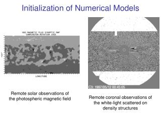
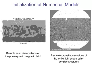
Initialization of Numerical Models Remote solar observations of the photospheric magnetic field Remote coronal observations of the white-light scattered on density structures
Observational evidence: • CME expands self-similarly • Angular extent is constant • Conceptual model: • CME as a shell-like region of enhanced density CME Cone Model [ Howard et al, 1982; Fisher & Munro, 1984 ] • Fitting of halo CMEs: • Various authors [Zhao, Liu, Michalek, Xie, etc] • Weak and fuzzy images • Cannot see “beyond” • STEREO will significantly improve accuracy
12 May 1997 1 May 1998 Application of the CME Cone Model 21 April 2002 24 August 2002 The heliospheric simulations may provide a global context of transient disturbances within a co-rotating, structured solar wind and they can serve as an intermediate solution until more sophisticated CME models become available.
Evolution of Parameters at Earth – Case A Poorly defined shock and its stand-off distance from the ejecta
Evolution of Parameters at Earth – Case B Accurate locations of stream boundaries and their rapid displacements are important for ICME properties at Earth
[ SAIC maps -- Pete Riley ] Effect of Fast-Stream Evolution Case A Case B Earth : Interaction region followed by shock and CME (not observed) Earth : Shock and CME (observed but shock front is radial)
[ WSA maps – Nick Arge ] Effect of Fast-Stream Evolution Case A Case B Earth : Interaction region followed by shock and CME (not observed) Earth : Shock and CME (observed but shock front is radial)
CMEs Cone Model Parameters CMEs fitted by:Liu (2005),Michalek (2003) and linear POS fit(CME list)
Magnetic Cloud and Fast Stream Post-Eruptive Flow MC Fast Stream Sudden Stream Displacement MC Fast Stream
Increasing Accuracy of Cone Model Specification STEREO-A ICME SUN EARTH STEREO-B
Geometric Localization of STEREO CMEs [ Pizzo and Biesecker, 2005 ]
Improving Validation of Cone Models – A Multi-point in-situ observations
Improving Validation of Cone Models – B Multi-point in-situ observations
May 12, 1997 Halo CME Running difference images fitted by the cone model
Case A Case B [ SAIC maps -- Pete Riley ] Fast-Stream Evolution Ambient state before the CME launch Disturbed state during the CME launch Ambient state after the CME launch
Cone Model Features Cone models – Intermediate solution until more realistic coronal models will enable routine application
Specification of Parameters Too many free parameters – while observed events may be reconstructed from case to case, their initialization cannot be automatized
Observed Ejecta Signatures and Shock Stand-off Interval Various interpretations of single-point, in-situ observations
WSA Model MAS Model UCSD Model Driving Heliospheric Computations at CCMC WSA Data MAS Data MAS Data UCSD Data In-Situ Data wsa2bc mas2bc mas2bc ucsd2bc coho2bc a3d2bc bnd.nc bnd.nc bnd.nc bnd.nc bnd.nc bnd.nc bnd.nc cone2bc ENLIL • Currently, there are three models (yellow) that can be used to drive ENLIL (green) • Computational system shares data sets (grey) and uses couplers (blue)
3-D Values at Time Level – tim.****.nc • Values are shown at Earth position (thick black line) and nearby grid points (light blue lines). • Observations from NASA-OMNIweb are shown by red dots. • Viewing evolution at nearby points can reveal effect of numerical resolution and can provide inclination of structures for geospace models • Values are shown on various slices passing through Earth • Current sheet is shown by white line • Planet positions are shown by black spheres • Calendar data and physical time correspond to file record number (****)