Time-Series Forecast Models
260 likes | 508 Vues
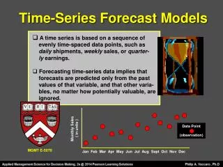
Time-Series Forecast Models. A time series is based on a sequence of evenly time-spaced data points, such as daily shipments, weekly sales, or quarter- ly earnings. Forecasting time-series data implies that forecasts are predicted only from the past

Time-Series Forecast Models
E N D
Presentation Transcript
Time-Series Forecast Models • A time series is based on a sequence of evenly time-spaced data points, such as daily shipments, weekly sales, or quarter- ly earnings. • Forecasting time-series data implies that forecasts are predicted only from the past values of that variable, and that other varia- bles, no matter how potentially valuable, are ignored. Data Point or (observation) Monthly Sales ( in units ) MGMT E-5070 Jan Feb Mar Apr May Jun Jul Aug Sept Oct Nov Dec
Decomposition of a Time Series • Analyzing time series means breaking down past data into components and then project- ing them into the future • A time series typically has four components: trend, seasonality, cycles, and randomvariation TIME SERIES MODELS ATTEMPT TO PREDICT THE FUTURE BY USING HISTORICAL DATA
Decomposition of a Time Series • Trend ( T )is the gradual upward or downward movement of the data over time. • Seasonality ( S )is a pattern of the demand fluc- tuation above or below the trend line that repeats at regular intervals. • Cycles ( C )are patterns in annual data that occur every several years. They are usually tied into the business cycle. • Random variations ( R )are blips in the data that are caused by chance and unusual situations. They follow no discernible pattern.
Time Series & Components SEASONAL PEAKS TREND COMPONENT AVERAGE DEMAND OVER 4 YEARS PRODUCT OR SERVICE DEMAND ACTUAL DEMAND LINE TIME YEAR 1 YEAR 2 YEAR 3 YEAR 4
Time Series & Components RANDOM VARIATIONS • Forecasters usually assume that the random variations are averaged out over time. • These random errors are often assumed to be normally distributed with a mean of zero. IT IS ALSO ASSUMED THAT RANDOM VARIATIONS DO NOT HEAVILY INFLUENCE DEMAND
The Moving Average Model • Assumes demand will stay fairly steady over time. • A two-month moving average forecast is found by summing the demand during the past two periods and dividing by “ 2 ” . • With each passing period, the most recent demand is added to the sum; the earliest demand is dropped. This smooths out short-term irregularities in the data series. • It has no trend, seasonal, or cyclical components.
The Moving Average Model Σ (demands in previous n periods ) n Forecast = n IS THE NUMBER OF PERIODS IN THE MOVING AVERAGE
The Moving Average Model TWO - PERIOD EXAMPLE 110 + 100 / 2 = 105 100 + 120 / 2 = 110 120 + 140 / 2 = 130
The Moving Average Model FOUR - PERIOD EXAMPLE 110 + 100 + 120 + 140 / 4 = 117.5 100 + 120 + 140 + 170 / 4 = 132.5
Weighted Moving Average Model • Makes the forecast more responsive to changes. • Used when there is a trend or pattern. Weights place more emphasis on recent values. • Deciding the weights requires some experience and good luck! SEVERAL WEIGHTS SHOULD BE TRIED, AND THE ONES WITH THE LOWEST FORECAST ERROR SHOULD BE SELECTED
Weighted Moving Average Model ∑ ( weight in period i )( actual value in period) ∑ ( weights )
Weighted Moving Average Model THREE - PERIOD 4th Period Forecast 8(120) + 1 (100) + 1 (110) = = 117 units 10 ‘10’ represents the sum of the weights
Weighted Moving Average Model THREE - PERIOD 5th Period Forecast 8(140) + 1 (120) + 1 (100) = = 134 units 10
Exponential Smoothing Model First Order or Primary Version A moving average technique that only requires the last period actual demand and the last period forecasted demand for input. THE NEW FORECAST α 1 - α LAST FORECASTED DEMAND LASTACTUALDEMAND = + The new forecast is equal to the old forecast adjusted by a fraction of the error ( last period actual demand – last period forecast ) . The smoothing coefficient ( α ) is a weight for the last actual demand.
Exponential Smoothing Example ASSUMING THAT α = .7 , THE NEXT FORECAST IS: .7 ( 100 units ) + ( 1 - .7 )( 110 units ) 70 + 33 = 103 units Last Actual Demand Last Forecast
Exponential Smoothing Example ASSUMING THAT α = .7 , THE NEXT NEW FORECAST IS: .7 ( 120 units ) + ( 1 - .7 )( 103 units ) 84 + 30.9 = 114.9 units Last Actual Demand Last Forecast
The Smoothing Coefficient • The symbol is alpha ( α ) • It can assume any value between 0 and 1 inclusive • It places a weight on the last actual period demand • The value of alpha resulting in the lowest forecast error is selected for the model.
Smoothing Coefficient Selection LOW - RANGE • This range ( .0 – .3 ) places the heaviest weight on the historical demand periods. • The intent is to make the forecast reflect the long - term stability of the product’s demand, as well as to minimize short-term fluctuations that could distort future forecasts. • It is appropriate for products whose demand patterns are extremely stable over time and expected to remain so.
Smoothing Coefficient Selection MEDIUM - RANGE • This range ( .4 – .6 ) splits weights between historical and most recent demand periods. • The intent is to make the forecast reflect the importance of each. • It is appropriate for products whose demand patterns are only slightlyunstable.
Smoothing Coefficient Selection HIGH - RANGE • This range ( .7 – 1.0 ) places the heaviest weight on the most recent demand periods. • The intent is to make the forecast largely reflect the most recent demand experience. • It is appropriate for products that are entirely new, and for products whose demand patterns are unstable.
Trend Projection Model A REGRESSION MODEL OVER TIME This technique fits a trend line through a series of historical data points and then projects that trend line into the future for both medium and long-range forecasting. WE WILL FOCUS ON STRAIGHT-LINE TRENDS FOR NOW
Trend Projection Model A REGRESSION MODEL OVER TIME We identify a straight line that minimizes the sum of the squares of the vertical distances from the regression line to each of the actual observations. THIS ALSO IMPLIES THAT THE MEAN SQUARED ERROR (MSE) IS MINIMIZED DEMAND ( Y ) THE TREND LINE MSE IS A MEASURE OF FORECAST ERROR TIME ( X )
Trend Projection Model Y-AXIS INTERCEPT : THE POINT ON THE VERTICAL AXIS THAT THE REGRESSION LINE CROSSES THE SLOPE OF THE LEAST-SQUARES LINE: THE RATE OF CHANGE IN ‘Y’ GIVEN CHANGE IN TIME ‘X’ ^ THE PREDICTED VALUE ( FORECAST ) THE SPECIFIED VALUE OF ‘X’ ( TIME ) Y = a + b X Y AXIS X AXIS ORIGIN
Trend Projection Model EXAMPLE 11th YEAR FORECAST Y - INTERCEPT SLOPE 11th YEAR ^ Y = a + b ( X ) ^ Y = 92.6667 + 10.9697 ( 11 ) 213.3333 units = 92.6667 + 120.6667