Common Trend Models for Time Series
This paper explores the application of common trend models, particularly Dynamic Factor Analysis (DFA) and Time Series Factor Analysis (TSFA), to time series data. It focuses on estimating underlying common trends among series like presidential approval ratings and tariff rates from Latin American countries. Insights on autocorrelation, model specification, and the consequences of nonstationarity are discussed, alongside practical implementations using statistical software. The findings enhance our understanding of how unobservable factors can impact measurable variables in political science and economics.

Common Trend Models for Time Series
E N D
Presentation Transcript
Common Trend ModelsforTime Series Jee-Kwang Park Post-Doctoral Fellow in QuaSSI Department of Political Science Pennsylvania State University
Factor Analysis • The object of interest is not directly observable (measurable) • But other seemingly related quantities are measurable • Factor analysis explain the correlations between measurable variables in terms of underlying factors, which are not directly measurable.
Factor Analysis • Ex) Mathematical abilities among students
Common trend Models(Dynamic Factor Analysis) • Estimate the underlying common trends among a group of time series. • Do factor analysis with time series • Estimate the factor loadings and predict factor scores • Business cycle, interest rates, stock prices • Three variants: DFA, TSFA, SSM
1) Dynamic Factor Analysis • Geweke (1977) first proposes the dynamic factor analysis • S-Plus/Finmetrics Program • DFA estimates the dynamics of the factors • Limit: valid with stationary series • most social science data are nonstationary
Time Series Factor Analysis (TSFA) • Gilbert and Meijer (2005) • P-technique factor analysis (Cattell et al) • works with nonstationary (weak bounded condition) • MLE, estimate is unbiased and consistent • Errors are not assumed to be iid • R package (tsfa)
State Space Model of Common Trends (SSM) • Engle and Watson(1981, 1983), Molenaar (1985), Harvey (1989), Lütkepohl(1991), Zuur (2003) • Works with nonstationary and short time series • can include explanatory variables • most widely used • Ox/STAMP
PresidentialApproval • 6 series : Gallup, ABC/WP, CBS/NYT, Fox, Pew, Zogby • Sources : www.pollingreport.com and roper center webpage • Monthly Presidential Approval Series • plural polls in a month, especially Gallup. • Averaging the plural polls is not so a good idea. • Cluster of polls, sample size
Presidential Approval • Missing Data • all polls but Gallup have missing months • (Cubic) spline smooth interpolation (Zivot & Wang 2002) • Spline ? nonparametric regression like Loess • Gallup = 0, Fox = 1, CBS/NYT = 4, ABC/WP = 9, Pew = 9, Zogby =12 missing observations
Presidential Approval • Previous Studies • Beck, (2006), Franklin (2006), Chung(2006)… • Franklin shows interesting findings on the house effects • CBS polls tend to fall 3% below the overall trend in 2005-2006: 38.2% 38.6% • Robert Chung’s finding : CBS polls have a small positive house effect during the pre-2005 period. • Autocorrelation (serial correlation)
Presidential Approval (DFA) • Using Finmetrics (S-Plus) • Wald test shows one common factor > factor.fit <- factanal(Bush.multiple, factors=1, method="mle") > factor.fit Sums of squares of loadings: Factor1 5.816041 … Test of the hypothesis that 1 factor is sufficient versus the alternative that more are required: The chi square statistic is 9.79 on 9 degrees of freedom. The p-value is 0.367
Presidential Approval (DFA) • 97% of variance is explained by one common factor > summary(factor.fit) Importance of factors: Factor1 SS loadings 5.8160408 Proportion Var 0.9693401 Cumulative Var 0.9693401 • Variance unique to each series The degrees of freedom for the model is 9. Uniquenesses: Gallup ABC/WP CBS Fox Pew Zogby 0.021 0.015 0.037 0.025 0.040 0.042
Presidential Approval (DFA) • Correlation among the polls > fitted(factor.fit) Gallup ABC CBS Fox Pew Zogby Gallup 1.000 0.981 0.970 0.976 0.968 0.967 ABC 0.981 0.999 0.973 0.979 0.971 0.970 CBS 0.970 0.973 0.999 0.968 0.961 0.960 Fox 0.976 0.979 0.968 0.999 0.966 0.965 Pew 0.968 0.971 0.961 0.966 0.999 0.958 Zogby 0.967 0.970 0.960 0.965 0.958 0.999
Presidential Approval (SSM) • The phenomenon conjectured by Franklin(2006) is supported by the residual plot • The same phenomenon is also visible in other polls
Presidential Approval (SSM) • Strength of SSM • We can compare a value in one series with one in another series due to following properties of SSM • 55% approval rate in Gallup is tantamount to 56.226% in ABC/WP poll. • ABC = .775*Gallup + 13.601+ error
Tariff Rates (DFA) • Tariff rates of 5 Latin American Countries • Missing observations • Two common factors • 80 % of variance is explained by 2 factors
Average Tariff Rates (SSM) • Two Common trends • Brazil seems to be best explained by the two common factors • Argentina is the worst fit, which means its tariff rates seem to be more influenced by domestic variables compared to the others. • The series co-moved more tightly in the second half of the period.
Conclusion • Common trends model will be useful - We have reason to believe multiple time series are influenced by the common factor(s) - The common factor cannot be directly measurable • We are interested in measuring the amount of the variances specific to each series • Another Application: asset returns model