Time Series Models
Time Series Models. Stochastic processes Stationarity White noise Random walk Moving average processes Autoregressive processes More general processes. Topics. Stochastic Processes. 1. Time series are an example of a stochastic or random process


Time Series Models
E N D
Presentation Transcript
Stochastic processes Stationarity White noise Random walk Moving average processes Autoregressive processes More general processes Topics
Time series are an example of a stochastic or random process A stochastic process is 'a statistical phenomenen that evolves in timeaccording to probabilistic laws' Mathematically, a stochastic process is an indexed collection of random variables Stochastic processes
We are concerned only with processes indexed by time, either discrete time or continuous time processes such as Stochastic processes
We base our inference usually on a single observation or realization of the process over some period of time, say [0, T] (a continuous interval of time) or at a sequence of time points {0, 1, 2, . . . T} Inference
To describe a stochastic process fully, we must specify the all finite dimensional distributions, i.e. the joint distribution of of the random variables for any finite set of times Specification of a process
A simpler approach is to only specify the moments—this is sufficient if all the joint distributions are normal The mean and variance functions are given by Specification of a process
Because the random variables comprising the process are not independent, we must also specify their covariance Autocovariance
Inference is most easy, when a process is stationary—its distribution does not change over time This is strict stationarity A process is weakly stationary if its mean and autocovariance functions do not change over time Stationarity
The autocovariance depends only on the time difference or lag between the two time points involved Weak stationarity
It is useful to standardize the autocovariance function (acvf) Consider stationary case only Use the autocorrelation function (acf) Autocorrelation
More than one process can have the same acf Properties are: Autocorrelation
This is a purely random process, a sequence of independent and identically distributed random variables Has constant mean and variance Also White noise
Start with {Zt} being white noise or purely random {Xt} is a random walk if Random walk
The random walk is not stationary First differences are stationary Random walk
Start with {Zt} being white noise or purely random, mean zero, s.d. Z {Xt} is a moving average process of order q (written MA(q)) if for some constants 0, 1, . . . q we have Usually 0 =1 Moving average processes
The mean and variance are given by The process is weakly stationary because the mean is constant and the covariance does not depend on t Moving average processes
If the Zt's are normal then so is the process, and it is then strictly stationary The autocorrelation is Moving average processes
Note the autocorrelation cuts off at lag q For the MA(1) process with 0 = 1 Moving average processes
In order to ensure there is a unique MA process for a given acf, we impose the condition of invertibility This ensures that when the process is written in series form, the series converges For the MA(1) process Xt = Zt + Zt - 1, the condition is ||< 1 Moving average processes
For general processes introduce the backward shift operator B Then the MA(q) process is given by Moving average processes
The general condition for invertibility is that all the roots of the equation lie outside the unit circle (have modulus less than one) Moving average processes
Assume {Zt} is purely random with mean zero and s.d. z Then the autoregressive process of order p or AR(p) process is Autoregressive processes
The first order autoregression is Xt = Xt - 1 + Zt Provided ||<1 it may be written as an infinite order MA process Using the backshift operator we have (1 – B)Xt = Zt Autoregressive processes
Autoregressive processes • From the previous equation we have
Autoregressive processes • Then E(Xt) = 0, and if ||<1
Autoregressive processes • The AR(p) process can be written as
This is for for some 1, 2, . . . This gives Xt as an infinite MA process, so it has mean zero Autoregressive processes
Conditions are needed to ensure that various series converge, and hence that the variance exists, and the autocovariance can be defined Essentially these are requirements that the i become small quickly enough, for large i Autoregressive processes
The i may not be able to be found however. The alternative is to work with the i The acf is expressible in terms of the roots i, i=1,2, ...p of the auxiliary equation Autoregressive processes
Then a necessary and sufficient condition for stationarity is that for every i, |i|<1 An equivalent way of expressing this is that the roots of the equation must lie outside the unit circle Autoregressive processes
Combine AR and MA processes An ARMA process of order (p,q) is given by ARMA processes
Alternative expressions are possible using the backshift operator ARMA processes
An ARMA process can be written in pure MA or pure AR forms, the operators being possibly of infinite order Usually the mixed form requires fewer parameters ARMA processes
General autoregressive integrated moving average processes are called ARIMA processes When differenced say d times, the process is an ARMA process Call the differenced process Wt. Then Wt is an ARMA process and ARIMA processes
Alternatively specify the process as This is an ARIMA process of order (p,d,q) ARIMA processes
The model for Xt is non-stationary because the AR operator on the left hand side has d roots on the unit circle d is often 1 Random walk is ARIMA(0,1,0) Can include seasonal terms—see later ARIMA processes
We have assumed that the mean is zero in the ARIMA models There are two alternatives mean correct all the Wt terms in the model incorporate a constant term in the model Non-zero mean
Outline of the approach Sample autocorrelation & partial autocorrelation Fitting ARIMA models Diagnostic checking Example Further ideas Topics
The approach is an iterative one involving model identification model fitting model checking If the model checking reveals that there are problems, the process is repeated Box-Jenkins approach
Models to be fitted are from the ARIMA class of models (or SARIMA class if the data are seasonal) The major tools in the identification process are the (sample) autocorrelation function and partial autocorrelation function Models
Use the sample autocovariance and sample variance to estimate the autocorrelation The obvious estimator of the autocovariance is Autocorrelation