Download
1 / 24
240 likes | 450 Vues
Other ISAs. Next, we discuss some alternative instruction set designs. Different ways of specifying memory addresses Different numbers and types of operands in ALU instructions End with fractional representations Fixed-point Floating-point. Addressing modes.

E N D
Other ISAs • Next, we discuss some alternative instruction set designs. • Different ways of specifying memory addresses • Different numbers and types of operands in ALU instructions • End with fractional representations • Fixed-point • Floating-point Other ISA's
Addressing modes • The first instruction set design issue we’ll see are addressing modes, which let you specify memory addresses in various ways. • Each mode has its own assembly language notation. • Different modes may be useful in different situations. • The location that is actually used is called the effective address. • The addressing modes that are available will depend on the datapath. • Our simple datapath only supports two forms of addressing. • Older processors like the 8086 have zillions of addressing modes. • We’ll introduce some of the more common ones. Other ISA's
Immediate addressing • One of the simplest modes is immediate addressing, where the operand itself is accessed. LD R1, #1999 R1 1999 • This mode is a good way to specify initial values for registers. • We’ve already used immediate addressing several times. Other ISA's
Direct addressing • Another possible mode is direct addressing, where the operand is a constant that represents a memory address. LD R1, 500 R1 M[500] • Here the effective address is 500, the same as the operand. • This is useful for working with pointers. • You can think of the constant as a pointer. • The register gets loaded with the data at that address. Other ISA's
Register indirect addressing • We already saw register indirect mode, where the operand is a register that contains a memory address. LD R1, (R0) R1 M[R0] • The effective address would be the value in R0. • This is also useful for working with pointers. In the example above, • R0 is a pointer, and R1 is loaded with the data at that address. • This is similar to R1 = *R0 in C or C++. • So what’s the difference between direct mode and this one? • In direct mode, the address is a constant that is hard-coded into the program and cannot be changed. • Here the contents of R0, and hence the address being accessed, can easily be changed. Other ISA's
Stepping through arrays • Register indirect mode makes it easy to access contiguous locations in memory, such as elements of an array. • If R0 is the address of the first element in an array, we can easily access the second element too: LD R1, (R0) // R1 contains the first element ADD R0, R0, #1 LD R2, (R0) // R2 contains the second element • This is so common that some instruction sets can automatically increment the register for you: LD R1, (R0)+ // R1 contains the first element LD R2, (R0)+ // R2 contains the second element • Such instructions can be used within loops to access an entire array. Other ISA's
Indexed addressing • Operands with indexed addressing include a constant and a register. LD R1, 500(R0) R1 M[R0 + 500] • The effective address is the register data plus the constant. For instance, if R0 = 25, the effective address here would be 525. • We can use this addressing mode to access arrays also. • The constant is the array address, while the register contains an index into the array. • The example instruction above might be used to load the 26th element of an array that starts at memory location 500. • It’s possible to use negative constants too, which would let you index arrays backwards. Other ISA's
PC-relative addressing • We’ve seen PC-relative addressing already. The operand is a constant that is added to the program counter to produce the effective memory address. 200: LD R1, $30 R1 M[201 + 30] • The PC usually points to the address of the next instruction, so the effective address here is 231 (assuming the LD instruction itself uses one word of memory). • This is similar to indexed addressing, except the PC is used instead of a regular register. • Relative addressing is often used in jump and branch instructions. • For instance, JMP $30lets you skip the next 30 instructions. • A negative constant lets you jump backwards, which is common in writing loops. Other ISA's
Indirect addressing • The most complicated mode that we’ll look at is indirect addressing. LD R1, [360] R1 M[M[360]] • The operand is a constant that specifies a memory location which refers to another location, whose contents are then accessed. • The effective address here is M[360]. • Indirect addressing is useful for working with multi-level pointers, or “handles.” • The constant represents a pointer to a pointer. • In C, we might write something like R1 = **ptr. Other ISA's
Addressing mode summary Other ISA's
Register transfer instruction: R0 R1 + R2 operation ADDR0, R1, R2 destination sources operands Number of operands • Another way to classify instruction sets is according to the number of operands that each data manipulation instruction can have. • Our example instruction set had three-address instructions, because each one had up to three operands—two sources and one destination. • This provides the most flexibility, but it’s also possible to have fewer than three operands. Other ISA's
Register transfer instruction: operation R0 R0 + R1 ADDR0, R1 source 2 operands destination and source 1 Two-address instructions • In a two-address instruction, the first operand serves as both the destination and one of the source registers. • Some other examples and the corresponding C code: ADD R3, #1 R3 R3 + 1 R3++; MUL R1, #5 R1 R1 * 5 R1 *= 5; NOT R1 R1 R1’ R1 = ~R1; Other ISA's
Register transfer instruction: operation source ACC ACC + R0 ADDR0 One-address instructions • Some computers, like this old Apple II, have one-address instructions. • The CPU has a special register called an accumulator, which implicitly serves as the destination and one of the sources. • Here is an example sequence which increments M[R0]: LD (R0) ACC M[R0] ADD #1 ACC ACC + 1 ST (R0) M[R0] ACC Other ISA's
The ultimate: zero addresses • If the destination and sources are all implicit, then you don’t have to specify any operands at all! • This is possible with processors that use a stack architecture. • HP calculators and their “reverse Polish notation” use a stack. • The Java Virtual Machine is also stack-based. • How can you do calculations with a stack? • Operands are pushed onto a stack. The most recently pushed element is at the “top” of the stack (TOS). • Operations use the topmost stack elements as their operands. Those values are then replaced with the operation’s result. Other ISA's
(Top) (Bottom) Stack architecture example • From left to right, here are three stack instructions, and what the stack looks like after each example instruction is executed. • This sequence of stack operations corresponds to one register transfer instruction: TOS R1 + R2 PUSH R1PUSH R2ADD Other ISA's
Data movement instructions • Finally, the types of operands allowed in data manipulation instructions is another way of characterizing instruction sets. • So far, we’ve assumed that ALU operations can have only register and constant operands. • Many real instruction sets allow memory-based operands as well. • We’ll use the book’s example and illustrate how the following operation can be translated into some different assembly languages. X = (A + B)(C + D) • Assume that A, B, C, D and X are really memory addresses. Other ISA's
Register-to-register architectures • Our programs so far assume a register-to-register, or load/store, architecture, which matches our datapath from last week nicely. • Operands in data manipulation instructions must be registers. • Other instructions are needed to move data between memory and the register file. • With a register-to-register, three-address instruction set, we might translate X = (A + B)(C + D) into: LD R1, A R1 M[A] // Use direct addressing LD R2, B R2 M[B] ADD R3, R1, R2 R3 R1 + R2 // R3 = M[A] + M[B] LD R1, C R1 M[C] LD R2, D R2 M[D] ADD R1, R1, R2 R1 R1 + R2 // R1 = M[C] + M[D] MUL R1, R1, R3 R1 R1 * R3 // R1 has the result ST X, R1 M[X] R1 // Store that into M[X] Other ISA's
Memory-to-memory architectures • In memory-to-memory architectures, all data manipulation instructions use memory addresses as operands. • With a memory-to-memory, three-address instruction set, we might translate X = (A + B)(C + D) into simply: • How about with a two-address instruction set? ADD X, A, B M[X] M[A] + M[B] ADD T, C, D M[T] M[C] + M[D] // T is temporary storage MUL X, X, T M[X] M[X] * M[T] MOVE X, A M[X] M[A] // Copy M[A] to M[X] first ADD X, B M[X] M[X] + M[B] // Add M[B] MOVE T, C M[T] M[C] // Copy M[C] to M[T] ADD T, D M[T] M[T] + M[D] // Add M[D] MUL X, T M[X] M[X] * M[T] // Multiply Other ISA's
Register-to-memory architectures • Finally, register-to-memory architectures let the data manipulation instructions access both registers and memory. • With two-address instructions, we might do the following: LD R1, A R1 M[A] // Load M[A] into R1 first ADD R1, B R1 R1 + M[B] // Add M[B] LD R2, C R2 M[C] // Load M[C] into R2 ADD R2, D R2 R2 + M[D] // Add M[D] MUL R1, R2 R1 R1 * R2 // Multiply ST X, R1 M[X] R1 // Store Other ISA's
Size and speed • There are lots of tradeoffs in deciding how many and what kind of operands and addressing modes to support in a processor. • These decisions can affect the size of machine language programs. • Memory addresses are long compared to register file addresses, so instructions with memory-based operands are typically longer than those with register operands. • Permitting more operands also leads to longer instructions. • There is also an impact on the speed of the program. • Memory accesses are much slower than register accesses. • Longer programs require more memory accesses, just for loading the instructions! • Most newer processors use register-to-register designs. • Reading from registers is faster than reading from RAM. • Using register operands also leads to shorter instructions. Other ISA's
Representing fractional numbers • Fixed-point numbers • Represent numbers using a fixed number of bits dedicated to the integer and fractional portion. • 10001001.0010110 - 8 bits each • .0111010010010101 – all 16 to the fractional portion • Frequently used in business applications • Evenly spaced gap between representable numbers for the full range. Other ISA's
Representing fractional numbers • Floating-point numbers • Somewhat similar to scientific notation • E.g. 1.001 x 2^13, 1.1 x 2^-4 • Several standards, most popular is the IEEE 754 • 32-bit float consists of: • 1 sign bit • 8 exponent bits • “excess-127” format. So treat bits as unsigned and subtract 127 from them to find actual exponents • 11111111 reserved to signify infinities and NaNs • 00000000 reserved to represent ‘denormalized’ numbers (no leading 1 assumed and e = -126) • 23 mantissa bits • Represent the fractional component, i.e. 1.01101 • Assume a leading 1 unless exponent is 0. • Value = -1s * 2(e-127) * 1.m Other ISA's
Representing fractional numbers • Floating-point numbers • IEEE 754 • 64-bit double-precision float consists of: • 1 sign bit • 11 exponent bits • “excess-1023” format. • 11111111 reserved to signify infinities and NaNs • 00000000 reserved to represent ‘denormalized’ numbers (no leading 1 assumed and e = -1022) • 52 mantissa bits • Represent the fractional component, i.e. 1.01101 • Assume a leading 1 unless exponent is 0. • Value = -1s * 2(e-1023) * 1.m • Uneven gaps between representable numbers (closer together when very small, larger gaps with larger numbers) Other ISA's
Summary • Instruction sets can be classified along several lines. • Addressing modes let instructions access memory in various ways. • Data manipulation instructions can have from 0 to 3 operands. • Those operands may be registers, memory addresses, or both. • Instruction set design is intimately tied to processor datapath design. Other ISA's