Download
1 / 27
280 likes | 552 Vues
Air Quality Management Chapter 5 Receptor Modeling for Air Quality Management. Ref: R.E. Hester and RM. Harrison, “Air Quality Management”, The Royal Society of Chemistry, Thomas Graham House, 1997. by Ping-hung Chen. Contents. 5.4 Secondary Arosol Mass 5.5 Apportionment of VOC.

E N D
Air Quality Management Chapter 5 Receptor Modeling for Air Quality Management Ref: R.E. Hester and RM. Harrison, “Air Quality Management”, The Royal Society of Chemistry, Thomas Graham House, 1997 by Ping-hung Chen
Contents 5.4 Secondary Arosol Mass 5.5 Apportionment of VOC
5.4 Secondary Arosol Mass Secondary Aerosol Mass The usual results of CMB analysis list ‘sulfate’ as a source or possibly describe it as ‘regional sulfate’ Similar results are typically obtained through factor analysis to develop effective control strategies necessary to attribute the secondary particle mass to the original gaseous precursor sources
5.4 Secondary Arosol Mass Spatial Analysis Examining the variation of a number of measured species in samples at a single site input data are the values of a single variable measured at a variety of sites at multiple times Thus, the analysis is seeking spatial and temporal variations of the measured variable Area of Influence analysis Malm et al. used EOF in addition to a trajectory based method
5.4 Secondary Arosol Mass SO2 sources Henry et al. used a modified EOF analysis to look for SO2 sources over the southwestern US Data are from 3 day long samples from the National Park Service sampling network Area of high positive values are likely source areas Negative values represent regions that serve as sulfur sinks
5.4 Secondary Arosol Mass Methods Incorporating Back Trajectories Potential Source Contribution Function (PSCF) Residence Time Analysis Air parcel has spent a given time within that grid cell Annular area/single grid cell area = pi[(Dij+L)^2 – (Dij-L)^2]/4L^2
5.4 Secondary Arosol Mass Residence Time Probability
5.4 Secondary Arosol Mass Areas of Influence Analysis Identifying those extreme samples at each measureement site Region was divided into 1o latitude by 1o longitude The extreme valued residence times will be highest around that site To eliminate this central tendency, deviding the residence time value by an equal probabilty residence time surface A new function assuming an air parcel can arrive at the receptor from any direction with equal probability This new function is the extreme source contribution function (ESCF)
5.4 Secondary Arosol Mass In AIA Identified source cells Calculated average ESCF for each receptor Plot cell values to locate the source Plot EOF results on the same map for comparison Figure 4 shows the AIA results
5.4 Secondary Arosol Mass AIA results
5.4 Secondary Arosol Mass EOF result
5.4 Secondary Arosol Mass Quantitative Bias Trajectory Analysis Lamb’s equation 3 A(x,t) = f(T, x,t) T(x,t)=f(Q, R,D,^) ---- equation 4 Q: probability of air parcel at x’ at t for receptor x ---- eq. 7 R: probability of material not lost by dry deposition D: proportional to Kd dry deposition --- eq. 5 ^: proportional to Kw wet deposition --- eq. 6
5.4 Secondary Arosol Mass Potential Source Contribution Function (PSCF) Both chemical and meteorological data for each filter sample are needed Eq. 12 P[Aij]=nij/N Eq. 13 P[Bij]=mij/N Eq. 14 Pij=P[Bij]/P[Aij]=mij/nij Pij is the conditional probability Sufficient number of endpoints should provide accurate estimates of the source locations
5.4 Secondary Arosol Mass PSCF map for SO2, Claremont, CA
5.4 Secondary Arosol Mass PSCF map for SO42-, Claremont, CA
5.4 Secondary Arosol Mass Emissions estimates for the SoCAB
5.4 Secondary Arosol Mass PSCF-based Source Apportionment Model PSCF is using mean value for the recptor cells No source apportionment Apportionment method Eq. 16 Rijx=PijxEijx + [My/Mx]PijyEijx
5.4 Secondary Arosol Mass PSCF-weighted emissions estimates for SO2 to SO42-
5.4 Secondary Arosol Mass PSCF-weighted emissions estimates for NOx to NOy
5.5 Apportionment of VOC Problems of identifying the emission source A large number of small sources and there can be dfficulties in obtaining representative source samples The methods depend only on the measured ambient data would be useful if they can identify source locations and apportion the VOCs to theose sources Wet and dry deposition and dispersion information is important
5.5 Apportionment of VOC Analysis begins with Eq. 17 Average C = [(sum of Cxt)/(sum of t)] Eq. 18 Cil = cl(Xil/average Xl) Simulation Iteration of the field Change is less than 0.5%
5.5 Apportionment of VOC Results The areas of high concentration are focused around the highway network particularly to the east of the downtown ring road Point source emissions Several specific areas to the southeast of the downtown area have high contributions to the measured concentrations
5.5 Apportionment of VOC Residence time weighted concentration for ethene
5.5 Apportionment of VOC Residence time weighted concentration for 2-methylpentane