Air Quality Modeling

1. Reading: Chap 7.3 Air Quality Modeling • Overview of AQ Models • Gaussian Dispersion Model • Chemical Mass Balance (CMB) Models

2. Overview

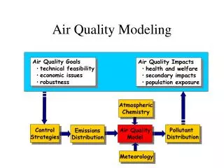
3. Overview What is the level of my exposure to these emissions? Is my family safe? Where is safe? How about the adverse impact on the environment (plants, animals, buildings)?How to predict the impact of emissions resulting from population growth? • Air Quality Models are mathematical formulations that include parameters that affect pollutant concentrations. They are used to • Evaluate compliance with NAAQS and other regulatory requirements • Determine extent of emission reductions required • Evaluate sources in permit applications

4. Meteorological Model Emission Model Chemical Model Temporal and spatial emission rates Topography Chemical Transformation Pollutant Transport Equilibrium between Particles and gases Vertical Mixing Source Dispersion Model Receptor Model Types of AQ Models

5. Emission Model • Estimates temporal and spatial emission rates based on activity level, emission rate per unit of activity and meteorology • Meteorological Model • Describes transport, dispersion, vertical mixing and moisture in time and space • Chemical Model • Describes transformation of directly emitted particles and gases to secondary particles and gases; also estimates the equilibrium between gas and particles for volatile species

6. Source Dispersion Model • Uses the outputs from the previous models to estimate concentrations measured at receptors; includes mathematical simulations of transport, dispersion, vertical mixing, deposition and chemical models to represent transformation. • Receptor Model • Infers contributions from different primary source emissions or precursors from multivariate measurements taken at one ore more receptor sites. When are model applications required for regulatory purposes?

7. Regulatory Application of Models • PSD: Prevention of Significant Deterioration of Air Quality in relatively clean areas (e.g. National Parks) • SIP: State Implementation Plan revisions for existing sources and to New Source Reviews (NSR)

8. Classifications of AQ Models • Developed for a number of pollutant types and time periods • Short-term models – for a few hours to a few days; worst case episode conditions • Long-term models – to predict seasonal or annual average concentrations; health effects due to exposure • Classified by • Non-reactive models – pollutants such as SO2 and CO • Reactive models – pollutants such as O3, NO2, etc.

9. AQ Models • Classified by coordinate system used • Grid-based • Region divided into an array of cells • Used to determine compliance with NAAQS • Trajectory • Follow plume as it moves downwind • Classified by level of sophistication • Screening: simple estimation use preset, worst-case meteorological conditions to provide conservative estimates. Purpose? • Refined: more detailed treatment of physical and chemical atmospheric processes; require more detailed and precise input data. So what? http://www.epa.gov/scram001/images/grid4.jpg http://www.epa.gov/scram001/images/smokestacks.jpg

10. USEPA AQ models • Screening models available at: http://www.epa.gov/scram001/dispersion_screening.htm • Preferred models available at: http://www.epa.gov/scram001/dispersion_prefrec.htm • A single model found to outperform others • Selected on the basis of other factors such as past use, public familiarity, cost or resource requirements and availability • No further evaluation of a preferred model is required • Alternative models available at: http://www.epa.gov/scram001/dispersion_alt.htm • Need to be evaluated from both a theoretical and a performance perspective before use • Compared to measured air quality data, the results indicate the alternative model performs better for the given application than a comparable preferred model • The preferred model is less appropriate for the specific application or there is no preferred model

11. USEPA AQ models

12. Gaussian Dispersion Models • Most widely used • Based on the assumption • plume spread results primarily by molecular diffusion • horizontal and vertical pollutant concentrations in the plume are normally distributed (double Gaussian distribution) • Plume spread and shape vary in response to meteorological conditions X Z Q u Y H Fig 7.11

13. Model Assumptions • Gaussian dispersion modeling based on a number of assumptions including • Steady-state conditions (constant source emission strength) • Wind speed, direction and diffusion characteristics of the plume are constant • Mass transfer due to bulk motion in the x-direction far outshadows the contribution due to mass diffusion • Conservation of mass, i.e. no chemical transformations take place • Wind speeds are >1 m/sec. • Limited to predicting concentrations > 50 m downwind

14. Gaussian Dispersion Equation Atmospheric Stability Classes Why isn’t x in the equation? Table 7.4

15. Dispersion Coefficients: Horizontal Fig 7.12

16. Dispersion Coefficients: Vertical Fig 7.13

17. Gaussian Dispersion Equation If the emission source is at ground level with no effective plume rise then Plume Rise • H is the sum of the physical stack height and plume rise.

18. Plume Rise Buoyant plume: Initial buoyancy >> initial momentum Forced plume: Initial buoyancy ~ initial momentum Jet: Initial buoyancy << initial momentum • For neutral and unstable atmospheric conditions, buoyant rise can be calculated by Vs: Stack exit velocity, m/s d: top inside stack diameter, m Ts: stack gas temperature, K Ta: ambient temperature, K g: gravity, 9.8 m/s2 where buoyancy flux is

19. When pollutants are dispersed to the ground level, how should we handle the situation? Carson and Moses: vertical momentum & thermal buoyancy, based on 615 observations involving 26 stacks. (heat emission rate, kJ/s) (stack gas mass flow rate. kg/s)

20. Wark & Warner, “Air Pollution: Its Origin & Control” What if the surface is absorbing? How should the concentration profile look like w/ reflection?

21. Ground level concentration

22. Maximum Ground Level Concentration Under moderately stable to near neutral conditions, The ground level concentration at the center line is The maximum occurs at Once szis determined, x can be known and subsequently C.

23. Example • An industrial boiler is burning at 12 tons (10.9 mton) of 2.5% sulfur coal/hr with an emission rate of 151 g/s. The following exist : H = 120 m, u = 2 m/s, y = 0. It is one hour before sunrise, and the sky is clear. Determine downwind ground level concentration at 10 km. Stability class = sy = sz = C(10 km, 0, 0) =

24. Exercise • If emissions are from a ground level source with H = 0, u = 4 m/s, Q = 100 g/s, and the stability class = B, what is downwind concentration at 200 m? At 200 m: sy = sz = C(200 m, 0, 0) =

25. Example • Calculate H using plume rise equations for an 80 m high source (h) with a stack diameter = 4 m, stack velocity = 14 m/s, stack gas temperature = 90o C (363K), ambient temperature = 25 oC (298K), u at 10 m = 4m/s, and stability class = B. Then determine MGLC at its location. F = h plume rise = H = sz = sy = Cmax = Residents around Florida Rock Cement Plant are complaining its emission being violating its allowed level. The plant has its facility within 0.5 km diameter. Its effective stack height is 60 m. You are a FLDEP environmental specialist. Where are you going to locate your air quality monitors? Why?

26. 8 2 6 7 9 1 13 14 11 3,4,5,12 10 Chemical Mass Balance Model • A receptor model for assessing source apportionment using ambient data and source profile data. • Available at EPA Support Center for Regulatory Air Models - http://www.epa.gov/scram001/tt23.htm PM10emissions from permitted sources in Alachua County (tons) (ACQ,2002) 2000 Values 1. GRU Deerhaven 144.2 2. Florida Rock cement plant 34.35 3. Florida Power UF cogen. plant 3.19 1997 Values 4. VA Medical Center incinerator 0.2 5. UF Vet. School incinerator 0.2 6. GRU Kelly 1.9 7. Bear Archery 9.5 8. VE Whitehurst asphalt plant 4.9 9. White Construction asphalt plant 0.7 10. Hipp Construction asphalt plant 0.3 11. Driltech equipment manufacturing 0.2 Receptor Sites 12. University of Florida 13. Gainesville Regional Airport 14. Gainesville Regional Utilities (MillHopper)

27. Principles Cij = Σ(aik×Skj) • Mass at a receptor site is a linear combination of the mass contributed from each of a number of individual sources; • Mass and chemical compositions of source emissions are conserved from the time of emission to the time the sample is taken. • Cij is the concentration of species ith in the sample jthmeasured at the receptor site: • aik is the mass fraction of the species in the emission from source kth, and • Skj is the total mass contribution from source kth in the jth sample at the receptor site.

28. Example • Total Pb concentration (ng/m3) measured at the site: a linear sum of contributions from independent source types such as motor vehicles, incinerators, smelters, etc PbT = Pbauto + Pb incin. + Pbsmelter +… • Next consider further the concentration of airborne lead contributed by a specific source. For example, from automobiles in ng/m3, Pbauto, is the product of two cofactors: the mass fraction (ng/mg) of lead in automotive particulate emissions, aPb, auto, and the total mass concentration (mg/m3) of automotive emission to the atmosphere, Sauto • Pbauto = aauto(ng/mg) × Sauto (mg/m3air)

29. Assumptions • Composition of source emissions is constant over period of time, • Chemicals do not react with each other, • All sources have been identified and have had their emission characterized, including linearly independent of each other, • The number of source category (j) is less than or equal to the number of chemical species (i) for a unique solution to these equations, and • The measurement uncertainties are random, uncorrelated, and normally distributed (EPA, 1990).

30. Quick Reflection