Air Quality Modeling
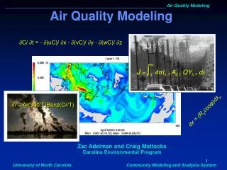
∞. J = ∫ 4 π I λ ,T A λ ,T QY λ ,T d λ. 0. Air Quality Modeling. ∂C/ ∂t = - ∂(uC)/ ∂x - ∂(vC)/ ∂y - ∂(wC)/ ∂z. kr = Ar(300/T)Bexp(Cr/T). dx = (R e cos φ )d λ e. Zac Adelman and Craig Mattocks Carolina Environmental Program. Outline. Why model air pollution?

Air Quality Modeling
E N D
Presentation Transcript
∞ J = ∫4πIλ,T Aλ,T QYλ,T dλ 0 Air Quality Modeling ∂C/ ∂t = - ∂(uC)/ ∂x - ∂(vC)/ ∂y - ∂(wC)/ ∂z kr = Ar(300/T)Bexp(Cr/T) dx = (Recosφ)dλe Zac Adelman and Craig MattocksCarolina Environmental Program
Outline • Why model air pollution? • Air quality modeling system components • Meteorology • Emissions • Chemistry and transport • Technical and operational details • Problems in air quality modeling • Application examples • Future directions in atmospheric modeling
Gas Chemistry: Aqueous Chemistry: O3 + NO NO2 + O2 SO2(g) SO2 (aq) O + O2 + M O3 + M Aerosol Processes: Condensation & Deposition Evaporation & Sublimation Nucleation & Coagulation Advection Diffusion Boundary Conditions Biogenic Emissions Anthropogenic Emissions Geogenic Emissions Adapted from Mackenzie and Mackenzie, “Our Changing Planet”, Prentice Hall, New Jersey, 1995. Source Sink
Why model air pollution? • Air pollution models are frameworks that integrate our understanding of individual processes with atmospheric measurements • Air pollution systems are non-linear • Need to establish the link between emissions sources and ambient concentrations
Air Quality Modeling Components • Meteorology modeling • Emissions processing • Initial/boundary conditions processing • Photolysis rate processing • Chemistry and transport modeling
WRF-ARW Basics • Fundamentals of Numerical Weather Prediction • Real vs. artificial atmosphere • Map projections • Horizontal grid staggering • Vertical coordinate systems • Definitions & Acronyms • Flavors of WRF • ARW core • NMM core • Other Numerical Weather Prediction Models • MM5 • ARPS • Global Icosahedral • WRF Model Governing Equations • Vertical coordinate and grid discretization • Time integration • Microphysics • Current Defects of WRF
Real vs. Artificial Atmosphere True analytical solutions are unknown! Numerical models are discrete approximations of a continuous fluid.
Map Projections Example of a regional high resolution grid (projection of a spherical surface onto a 2D plane) nested within a global (lat,lon) grid with spherical coordinates x = r cos y = r Differences in map projections require caution when dealing with flow of information across grid boundaries. WRF offers polar stereographic, Lambert conformal, Mercator and rotated Lat-Lon map projections.
Arakawa “A” Grid • Unstaggered grid - all variables defined everywhere. • Poor performance, first grid geometry employed in NWP models. • Noisy - large errors, short waves propagate energy in wrong direction, additional smoothing required. • Poorest at geostrophic adjustment - wave energy trapped, heights remain too high. • Can use a 2x larger time step than staggered grids.
Arakawa “B” Grid • Staggered, velocity at corners. • Preferred at coarse resolution. • Superior for poorly resolved inertia-gravity waves. • Good for geostrophy, Rossby waves: collocation of velocity points. • Bad for gravity waves: computational checkerboard mode. • Used by MM5 model.
Arakawa “C” Grid • Staggered, mass at center, normal velocity, fluxes at grid cell faces, vorticity at corners. • Preferred at fine resolution. • Superior for gravity waves. • Good for well resolved inertia-gravity waves. • Simulates Kelvin waves (shoulder on boundary) well. • Bad for poorly resolved waves: Rossby waves (computational checkerboard mode) and inertia-gravity waves due to averaging the Coriolis force. • Used by WRF-ARW, ARPS, CMAQ models.
Arakawa “D” Grid • Staggered, mass at center, tangential velocity along grid faces. • Poorest performance, worst dispersion properties, rarely used. • Noisy - large errors, short waves propagate energy in wrong direction.
Arakawa “E” Grid • Semi-staggered grid. • Equivalent to superposition of 2 C-grids, then rotated 45 degrees. • Center set to translated (lat,lon) = (0,0) to prevent distortion near edges, poles. • Developed for Eta step-mountain coordinate to enhance blocking, overcome PGF errors caused by sigma coordinates. • Controls the cascade of energy toward smaller scales. • Used by WRF-NMM and Eta models.
Definitions & Acronyms • WRF: Weather Research & Forecasting numerical weather prediction model • ARW: Advanced Research WRF [nee Eulerian Model (EM)] core • NMM: Nonhydrostatic Mesoscale Model core • WRF-SI: Standard Initialization (4 components) - prepares real atmospheric data for input to WRF • WRF-VAR: Variational 3D/4D data assimilation system (not used for this class) • IDV: Integrated Data Viewer - Java application for interactive visualization of WRF model output
Flavors of WRF (ARW) • ARW solver (research - NCAR, Boulder, Colorado) • Fully compressible, nonhydrostatic equations with hydrostatic option • Arakawa-C horizontal grid staggering • Mass-based terrain following vertical coordinate • Vertical grid spacing can vary with height • Top is a constant pressure surface • Scalar-conserving flux form for prognostic model variables • 2nd to 6th-order advection options in horizontal &vertical • One-way, two-way and movable nest options • Runge-Kutta 2nd & 3rd-order time integration options • Time-splitting • Large time step for advection • Small time step for acoustic and internal gravity waves • Small step horizontally explicit, vertically implicit • Divergence damping for suppressing sound waves • Full physics options for land surface, PBL, radiation, microphysics and cumulus parameterization • WRF-chem under development: http://ruc.fsl.noaa.gov/wrf/WG11/
Flavors of WRF (NMM) • NMM solver (operational - NCEP, Camp Springs, Maryland) • Fully compressible, nonhydrostatic equations with reduced hydrostatic option • Arakawa-E horizontal grid staggering, rotated latitude-longitude • Hybrid sigma-pressure vertical coordinate • Conservative, positive definite, flux-corrected scheme used for horizontal and vertical advection of TKE and water species • 2nd-order spatial that conserves a number of 1st-order and quadratic quantities, including energy and enstrophy • One-way, two-way and movable nesting options • Time-integration schemes: forward-backward for horizontally propagating fast waves, implicit for vertically propagating sound waves, Adams-Bashforth for horizontal advection and Coriolis force, and Crank-Nicholson for vertical advection • Divergence damping & E subgrid coupling for suppressing sound waves • Full physics options for land surface, PBL, radiation, microphysics (only Ferrier scheme) and cumulus parameterization • Note: Many ARW core options are not yet implemented! Nesting still under development • NMM core will be used for HWRF (hurricane version of WRF), operational in summer of 2007
Other NWP Models (MM5) • MM5 (research - PSU/NCAR, Boulder, Colorado) • Progenitor of WRF-ARW, mature NWP model with extensive configuration options • Support terminated, no future enhancements by NCAR’s MMM division • Nonhydrostatic and hydrostatic frameworks • Arakawa-B horizontal grid staggering • Terrain following sigma vertical coordinate • Unsophisticated advective transport schemes cause dispersion, dissipation, poor mass conservation, lack of shape preservation • Outdated Leapfrog time integration scheme • One-way and two-way (including movable) nesting options • 4-dimensional data assimilation via nudging (Newtonian relaxation), 3D-VAR, and adjoint model • Full physics options for land surface, PBL, radiation, microphysics and cumulus parameterization
Other NWP Models (ARPS) • ARPS (research - CAPS/OU, Norman, Oklahoma) • Advanced Regional Prediction System • Sophisticated NWP model with capabilities similar to WRF • Primarily used for tornado simulations at ultra-high (25 meter) resolutions and assimilation of experimental radar data at mesoscale • Elegant, source code, easy to read/understand/modify, ideal for research projects, very helpful scientists at CAPS • Arakawa-C horizontal grid staggering • Currently lacks full mass conservation and Runge-Kutta time integration scheme • ARPS Data Assimilation System (ADAS) under active development/enhancement (MPI version soon), faster & more flexible than WRF-SI, employed in LEAD NSF cyber-infrastructure project • wrf2arps and arps2wrf data set conversion programs available • http://www.caps.ou.edu/ARPS/arpsdownload.html
WRF Model Governing Equations(Eulerian Flux Form) Momentum: ∂U/∂t + (∇ · Vu) − ∂(pφη)/∂x + ∂(pφx)/∂η = FU ∂V/∂t + (∇ · Vv) − ∂(pφη)/∂y + ∂(pφy)/∂η = FV ∂W/∂t + (∇ · Vw) − g(∂p/∂η − μ) = FW Potential Temperature: Diagnostic Hydrostatic (inverse density a): ∂Θ/∂t + (∇ · Vθ) = FΘ ∂φ/∂η = -μ Continuity: where: μ = column mass V = μv = (U,V,W) Ω = μ d(η)/dt Θ = μθ ∂μ/∂t + (∇ · V) = 0 Geopotential Height: ∂φ/∂t + μ−1[(V · ∇φ) − gW] = 0
Runge-Kutta Time Integration Φ∗ = Φt + t/3 R(Φt ) Φ∗∗ = Φt + t/2 R(Φ∗) Φt+t = Φt + t R(Φ∗∗) “2.5” Order Scheme Linear: 3rd order Non-linear: 2nd order Square Wave Advection Tests:
Runge-Kutta Time Step Constraint • RK3 is limited by the advective Courant number (ut/x) and the user’s choice of advection schemes (2nd through 6th order) • The maximum stable Courant numbers for advection in the RK3 scheme are almost double those in the leapfrog time-integration scheme Maximum Courant number for 1D advection in RK3
Microphysics • Includes explicitly resolved water vapor, cloud and precipitation processes • Model accommodates any number of mixing-ratio variables • Four-dimensional arrays with 3 spatial indices and one species index • Memory (size of 4th dimension) is allocated depending on the scheme • Carried out at the end of the time-step as an adjustment process, does not provide tendencies • Rationale: condensation adjustment should be at the end of the time step to guarantee that the final saturation balance is accurate for the updated temperature and moisture • Latent heating forcing for potential temperature during dynamical sub-steps (saving the microphysical heating as an approximation for the next time step) • Sedimentation process is accounted for, a smaller time step is allowed to calculate vertical flux of precipitation to prevent instability • Saturation adjustment is also included
WRF Microphysics Options • Mixed-phase processes are those that result from the interaction of ice and water particles (e.g. riming that produces graupel or hail) • For grid sizes ≤ 10 km, where updrafts may be resolved, mixed-phase schemes should be used, particularly in convective or icing situations • For coarser grids the added expense of these schemes is not worth it because riming is not likely to be resolved
Current Defects of WRF • Serious deficiencies in PBL parameterizations and land surface models produce biases/errors in the predicted surface and 2-meter temperatures, and PBL height. WRF cannot maintain shallow stable layers. • 3D/4D Variational data assimilation and Ensemble Kalman Filtering (EnKF) still under development, EnKF available to community from NCAR as part of the Data Assimilation Research Testbed (DART). • Not clear yet what to do in “convective no-man’s land” – convective parameterizations valid only at horizontal scales > 10 km, but needed to trigger convection at 5-10 km scales. • Multi-species microphysics schemes with more accurate particle size distributions and multiple moments should be developed to rectify errors in the prediction of convective cells. • Heat and momentum exchange coefficients need to be improved for high-wind conditions in order to forecast hurricane intensity. Wind wave and sea spray coupling should also be implemented. Movable, vortex-following 2-way interactive nested grid capability has recently been incorporated into the WRF framework. • Upper atmospheric processes (gravity wave drag and stratospheric physics) need to be improved for coupling with global models.
Emissions Processing Area Mobile Point Biogenic • Emissions Processing Steps AQM-ready Emissions:
Emissions Terminology • Inventory: estimate of pollutant emissions at a given spatial unit • Model Grid: 3-d representation of the earths surface based on discrete and uniform spatial units, i.e. grid cells • Speciation: conversion of inventory pollutant species to model pollutant species • Gridding: conversion of inventory spatial units to model grid cells • Temporalization: conversion of inventory temporal units to those requires by an air quality model
Emissions Terminology • Plume rise: calculation of the vertical distribution of emissions from point sources and the subsequent allocation of the emissions to the model layers • Spatial surrogate: GIS-based estimate of the fraction of a grid cell covered by a particular land-use category (e.g. population or rural housing) • Profiles: emissions distributions in space, time, or to chemical species • Cross-referencing: relating profiles to specific emissions sources
Area sources • Most basic inventory unit • Country/province/municipality wide estimate • Requires spatial surrogates to map to a model grid • Examples • Construction and agricultural emissions • Road dust • Fires
Mobile sources • On-road: Estimate by road way and vehicle type • Requires emissions factors for local vehicles and activities/speeds for local roads • Gridding by road way distribution or links • Can use local meteorology to adjust emissions factors for temperature and humidity • Examples: Heavy-duty diesel trucks on primary highways, light-duty gasoline cars on rural roads • Non-road: Area-like estimates • Examples: Construction and mining vehicles, recreational vehicles (boats, ATV’s),
Point sources • Emissions at specific latitude-longitude coordinates • Often elevated sources that require stack parameters (e.g. stack height, exit gas velocities, exit gas temperatures, etc.) • Can use annual, daily, or hourly emissions estimates • Examples: • Electricity generating units (EGU’s) • Smelters • Wildfires
Biogenic sources • Estimates of emissions from vegetation and soils • Uses gridded land-use data and emissions factors by vegetation type • Uses local meteorology to calculate emissions based on photosynthetically active radiation (PAR) and to adjust for temperatures • Examples: • VOC emissions from specific tree species • Soil NO
Gridded sources • Pre-gridded emissions from global databases • Normalize to the model grid to combine with other sources • Can encompass any of the emissions categories • Top-down vs. bottom-up emissions estimate
Emissions Processing • Purpose: convert emissions data to formats required by air quality model • Primary functions • Import data into system • Spatial allocation (gridding) • Chemical allocation (speciation) • Temporal allocation • Merge • Quality assurance
Data Import Inventory categories Area Point Mobile Biogenic Gridded ASCII or gridded binary Country/state/county estimates Annual estimates Pollutants include bulk VOC and PM2.5 Spatial Allocation Inventory spatial units model grid Requires spatial surrogates Emissions Processing Steps EI Grid Cell Mapping
Chemical Allocation Tons Moles Converts inventory pollutants to air quality model species Model-dependent speciation profiles NOx NO + NO2 VOC PAR, OLE, etc. PM2.5 NO3, SO4, etc. Temporal allocation Inventory units hourly emissions Requires temporal profiles Emissions Processing Steps Monthly Weekly Diurnal
Merging Combine all intermediate steps to create AQM-ready emissions Combine individual source categories Formatting Units Output file naming Quality Assurance Report base inventory values and changes at each processing step Customize reporting e.g. by state and SCC, by SCC and temporal profiles, by grid cell and surrogate I.D. Means to determine why a result occurred Emissions Processing Steps
Plume Rise Allocate elevated emissions sources to vertical model layers Compute layer fractions Require meteorology to calculate plume buoyancy Stationary point, fires, in-flight aircraft Projections Grow and/or control inventories for future year modeling Source-based projection information Other Emissions Processing Steps
Import Grid Speciate Temporal Merge Grid Speciate Import Merge Temporal Emissions Processing Paradigms • Linear • Sequential steps that follow a particular order • Requires completing one step before completing the next • Parallel • Flexible sequence with steps in any order AQM AQM
Initial and Boundary Conditions • Initial conditions define the chemical conditions at the start of a simulation • Defined using vertical profiles of clean background concentrations • Boundary conditions define the chemical conditions on the horizontal faces of the modeling domain • Static and dynamic boundaries are possible • Initial conditions decay exponentially with simulation time; boundary conditions on the upwind boundary continue to affect predictions through an entire simulation.
Initial/Boundary Condition Processing • Processing requires generating IC/BC estimates on a model-grid • Nested simulations extract BC’s from a parent grid • Multi-day simulations extract IC’s from the last hour of the previous day
∞ J = ∫4πIλ,T Aλ,T QYλ,T dλ 0 Photolysis Rate Processing • Photolysis: Chemical dissociation caused by the absorption of solar radiation • Photolysis rate: rate of reaction for pollutants that undergo photolysis • Processing calculates clear sky photolysis rates at different latitudes and altitudes • Air quality models adjust rates with cloud cover estimates from meteorology
What are air quality models? • Statistical models: describe concentrations in the future as a statistical function of current chemical and/or meteorological conditions • Chemistry-transport models (CTM): based on fundamental descriptions of physical and chemical processes in the atmosphere
How do CTMs work? • Air Quality Model processes • Dynamical/thermodynamical: meteorology, land surface conditions (soil, water) • Transport: emissions, advection, diffusion, dry deposition, sedimentation • Gas phase chemistry: photochemistry, phase changes • Radiative: optical depth, visibility, energy transfer • Aerosol/clouds: nucleation, coagulation, heterogeneous chemistry, aqueous chemistry
Lagrangian/Trajectory Models Moves relative to the coordinate Different locations at different times Only emissions enter the cell No material leaves the cell Overlay 3-D boxes on a grid