Download
1 / 15
150 likes | 252 Vues
Effective conductivity of collisionless plasma. Semenov, V. St. Petersburg University, Russia Divin , A. K. U. Leuven, Belgium Thanks to N. Erkaev , I. Kubyshkin , G. Lapenta , S. Markidis , and H. Biernat. Motivation.

E N D
Effective conductivity of collisionless plasma Semenov, V. St. Petersburg University, Russia Divin, A. K. U. Leuven, Belgium Thanks to N. Erkaev, I. Kubyshkin, G. Lapenta, S. Markidis, and H. Biernat
Motivation • Magnetic reconnection is one of the most important energy conversion process in various plasmas. • The process is determined by the presence of some sort of diffusivity in plasma, which breaks the magnetic field lines frozen-in constraint. • In collisionless plasma environments the problem of dissipation is not (yet) clear and several mechanisms are proposed (turbulent or laminar)
From global scales to EDR / History • Collisionless plasma: no collisional dissipation, but… • Turbulent: anomalous resistivity, wave-particle interaction • Laminar: electron inertia ? di de ~10…500 km (magnetotail) From: [Hesse, 2001]
Model parameters • Harris equilibrium, L=0.5di ,Ti/Te = 5, localized X-point perturbation Ay =Ay0 cos(2x/Lx )cos( z/Lz )exp(-(x2+z2)/a2) • Variables are normalized to initial CS parameters: n0, B0, VA, di, etc. • Bz(t=0)=0 • Runs reported: mi/me=1836, c/vA= 274, L= 40dix20di, (1024x512) 2048 p. mi/me=256, c/vA= 102, Ti/Te = 5, L= 200dix30di (2048x386) 940 p. mi/me=64, c/vA= 51, Ti/Te = 5, L= 20dix10di (512x256), 32 p. • We use the following magnetotail parameters as a reference (e.g. Pritchett, 2004): B0~20 nT, n0~0.3 cm-3 , Ωci-1~0.5s, c/pi~400km,vA~800km/s, EA=(vA/c)B0~16mV/m
Diffusion region: Ohm’s law На расстоянии ~4diот Х-линии: <1di Le внешняя EDR (выхлоп) внутренняя EDR На Х-линии Center of the EDR, Ey ~ -(1/ne)(dPyz/dz)y Edges of the EDR, Ey = (ve XB)y Anisotropy of electron pressure (mostly Peyz) supports Ez near X-point (in agreement with, see e.g. [Kuznetsova, 2000], [Pritchett, 2001])
Vz Vz Vy Vy naccvyacc n1 v1z Generation of Pyz n1 v1z naccvyacc
Sweet-Parker analysis: Results • EDR width: electron inertial length • Outflow velocity vx, electron Alfven • Reconnection rate (Ey/EA) connects all other parameters. Pressure-tensor based dissipation scales as Bohm diffusion !
Scaling: comparison to simulations (1) mi/me=256 (--), (ve x B)y (--), div Pe /(ne) (--), Ey (--), Vex (--), Vey (--), VeA (--),EDR width (--) local de estimate t/tA x/di
Scaling: comparison to simulations (2) mi/me=1836
Rescaling di de
Rescaling • The scaling implies that Larmor gyroradius • Simulations reveal that • This ratio is introduced into scaling:
Scaling: comparison to simulations (2) mi/me=1836
Rescaling mi/me=256 k=0.3
Rescaling mi/me=1836 k=0.3
Summary & Results • Magnetic reconnection is investigated by means of PIC simulations. • Study of EDR structure is performed and model for the pressure anisotropy is developed. • Sweet-Parker-like analysis of the EDR is performed; • All typical EDR parameters are recovered, diffusivity scales as Bohm diffusion. Rescaled equations are presented Vy =VAe z Ey VAe vy Vx =kVAe de