Power Laws
Power Laws. By Cameron Megaw 3/11/2013 . What is a Power Law?. A power law is a distribution of the form: similarly Example: The size of cities in the US (population 1000 or more) Highly right skewed The largest city has 8 million people Most cities have much fewer people.


Power Laws
E N D
Presentation Transcript
Power Laws By Cameron Megaw 3/11/2013
What is a Power Law? • A power law is a distribution of the form: • similarly • Example: The size of cities in the US (population 1000 or more) • Highly right skewed • The largest city has 8 million people • Most cities have much fewer people
Measuring Power LawsSampling Errors • 1 million random numbers from a power law distribution • Exponent • Data is binned in intervals of size .1 • Linear scales produce a smooth curve • Log-log scales have noisy data in the tail • Result of sampling errors • Corresponding bins have few samples (if any) • Fractional fluctuations in the bin counts are large
Measuring Power LawsSampling errors Solution 1: Throw out the data in the tail of the curve • Statistically significant information lost • Some distributions only follow a power law distribution in their tail • Not recommended
Measuring Power LawsSampling errors Solution 2: Very the width of the bins • Normalize the data • Results in a count per unit interval of x • Very bin size by a fixed multiplier (for example 2) • Bins become: 1 to 1.1, 1.1 to 1.3, 1.3 to 1.7 and so on • Called logarithmic binning
Measuring Power LawsSampling errors Solution 3: Calculate the probability distribution function (aka Zipf’s Law or a Pareto distribution) • No need to bin the data • Information on individual values are preserved • Eliminates the noise in the tail
Measuring Power LawsUnknown exponent • Method of least squares: • Most common method • Plots the line of best fit in log-log scales • Introduces systematic biases in the value of the exponent • Estimated (actual 2.5) • Use maximum likelihood formula • A non-biased estimator • Calculate an error estimate • standard bootstrap resampling • jackknife resampling • Estimated
Mathematics of Power LawsMoments • All moments exists for and diverge otherwise: • Mean: • Variance: • Intensity of Solar flares have an exponent 1.4 is the average intensity infinite? • All data sets have finite upper bound • Larger sampling space gives a non-negligible chance of increasing the upper bound
Mathematics of Power LawsLargest Value For a sample of size n we can estimate the largest value in the sample: as Where B is beta-function This estimate enables the calculation of moments for data sets whose moments would otherwise diverge.
Mathematics of Power LawsScale Free Distribution • A function is said to be scale free if: • The unit of measure does not affect the shape of the distribution • If 2kB files are as common as 1kB files then 2mB files are as common as 1mb files • Scale free distribution is unique to Power Law distributions • Scale free implies power law and vice versa
Mechanisms for Generating Power Laws Some examples : • Combinations of exponents • Inverses of quantities • Random Walks • The Yule process • Critical phenomena
The Topology of the InternetSome Key Questions What does the internet look like? Are there any topological properties that stay constant in time? How can I generate Internet-like graphs for simulation?
Internet Instances • Three Inter-domain topologies • November 1997, April and December 1998 • One Router topology from 1995
Outdegree of a Node and it’s Rank Power Law 1: The out degree of a nodev is proportional to the rank of the node, to the power of a constant R. By setting it can be shown that
Outdegree of a Node and it’s Rank • Inter domain topologies • Correlation coefficient above .974 • Exponents -.81, -.82, -.74 • Router • Correlation coefficient .948 • Exponent -.48
Outdegree and it’s Rank Power Law Analysis • The exponent is relatively fixed for the three inter-domain topologies • Topological property is fixed in time • Can be used to generate models or test authenticity • Significant difference in exponent value for the router topology • Can characterize different families of graphs • The rank exponent can be used to estimate the number of edges
Frequency of the Outdegree Power Law 2: The frequency, of an outdegree, d, is proportional to the outdegree to the power :
Frequency of the Outdegree • Inter domain topologies • Correlation coefficient above .968 • Exponents -2.15, -2.16, and -2.2 • Router • Correlation coefficient .966 • Exponent -2.48
Frequency of the Outdegree Power Law Analysis • The exponent is relatively fixed for the three inter-domain topologies • Topological property is fixed in time • Could be used to generate models or test authenticity • Similar exponent value for the router topology • Could suggest a fundamental property of the network
Eigenvalues and their Ordering • Power Law 3: The eigenvalues, of a graph are proportional to the order, • to the power of a constant :
Eigenvalues and their Ordering • Inter domain topologies • Correlation coefficient .99 • Exponents -.47, -.50, and -.48 • Router • Correlation coefficient .99 • Exponent -.1777
Eigenvalues and their Ordering Power Law analysis • Eigenvalues are closely related to many topological properties • Graph diameter • Number of edges • Number of spanning trees… • The exponent is relatively fixed for the three inter-domain topologies • Topological property seems fixed in time • Can be used to generate models • Significant difference in the exponent value for the router topology • Can characterize different families of graphs
Hop Plot Exponent • Approximation 1: The total number of pairs of nodes, within hops can be approximated by: • Where
Hop Plot Exponent • Inter domain topologies • First 4 hops • Correlation coefficient above .96 • Exponents -4.6, -4.7, -4.86 • Router • First 12 hops • Correlation coefficient .98 • Exponent -2.8
Hop Plot Exponent Power Law analysis • The exponent is relatively fixed for the three inter-domain topologies • Topological property seems fixed in time • Can be used to generate models • Significant difference in the exponent value for the router topology • Can characterize different families of graphs
The Effective Diameter How many hops to reach a “sufficiently large” part of the network? • Too small a broadcast will not reach the target • Too large a broadcast can clog the network • A good guess is the intersection of the hop-plot at The effective diameter For the interdomain instances • 80% of nodes were within • 90% were within
Average Neighborhood Size Average outdegree: Hop-plot exponent:
Conclusions Power Law and Internet topology • Can assess realism of synthetic graphs • Provide important parameters for graph generators • Help with network protocols • Help answer “what if” questions • What would the diameter be if the number of nodes doubles? • What would be the average neighborhood size be?