Lecture 15 - Discrete Phase Modeling Applied Computational Fluid Dynamics
530 likes | 1.77k Vues
Lecture 15 - Discrete Phase Modeling Applied Computational Fluid Dynamics. Instructor: André Bakker. © André Bakker (2002-2004) © Fluent Inc. (2002). Discrete phase modeling. Particle tracking. Steady vs. unsteady. Coupled vs. uncoupled. Advantages and limitations. Time stepping.

Lecture 15 - Discrete Phase Modeling Applied Computational Fluid Dynamics
E N D
Presentation Transcript
Lecture 15 - Discrete Phase ModelingApplied Computational Fluid Dynamics Instructor: André Bakker © André Bakker (2002-2004) © Fluent Inc. (2002)
Discrete phase modeling • Particle tracking. • Steady vs. unsteady. • Coupled vs. uncoupled. • Advantages and limitations. • Time stepping. • Discretization. Particle trajectories in a cyclone Particle trajectories in a spray dryer
Trajectories of particles/droplets are computed in a Lagrangian frame. Exchange (couple) heat, mass, and momentum with Eulerian frame gas phase. Discrete phase volume fraction should preferably be less than 10%. Mass loading can be large (+100%). No particle-particle interaction or break up. Turbulent dispersion modeled by: Stochastic tracking. Particle cloud model. Model particle separation, spray drying, liquid fuel or coal combustion, etc. continuous phase flow field calculation particle trajectory calculation update continuous phase source terms Discrete phase model
typical continuous phase control volume mass, momentum and heat exchange DPM theory Trajectory is calculated by integrating the particle force balance equation: Additional forces: Pressure gradient Thermophoretic Rotating reference frame Brownian motion Saffman lift Other (user defined) drag force is a function of the relative velocity Gravity force
Coupling between phases • One-way coupling: • Fluid phase influences particulate phase via drag and turbulence. • Particulate phase has no influence on the gas phase. • Two-way coupling: • Fluid phase influences particulate phase via drag and turbulence. • Particulate phase influences fluid phase via source terms of mass, momentum, and energy. • Examples include: • Inert particle heating and cooling. • Droplet evaporation. • Droplet boiling. • Devolatilization. • Surface combustion.
Particle types • Particle types are inert, droplet and combusting particle.
Heat and mass transfer to a droplet Temperature Tb Tv Tinjection Inert heating law Vaporization law Boiling law particle time
volatile fraction flashes to vapor Escape Trap Reflect Particle-wall interaction • Particle boundary conditions at walls, inlets, and outlets: • For particle reflection, a restitution coefficient e is specified:
Particle fates • “Escaped” trajectories are those that terminate at a flow boundary for which the “escape” condition is set. • “Incomplete” trajectories are those that were terminated when the maximum allowed number of time steps was exceeded. • “Trapped” trajectories are those that terminate at a flow boundary where the “trap” condition has been set. • “Evaporated” trajectories include those trajectories along which the particles were evaporated within the domain. • “Aborted” trajectories are those that fail to complete due to numerical/round-off reasons. If there are many aborted particles, try to redo the calculation with a modified length scale and/or different initial conditions.
Turbulence: discrete random walk tracking • Each injection is tracked repeatedly in order to generate a statistically meaningful sampling. • Mass flow rates and exchange source terms for each injection are divided equally among the multiple stochastic tracks. • Turbulent fluctuations in the flow field are represented by defining an instantaneous fluid velocity: • where is derived from the local turbulence parameters: • and is a normally distributed random number.
Stochastic tracking turned on. Five tracks per injection point. Adds random turbulent dispersion to each track. Tracks that start in the same point are all different. Stochastic tracking turned off. One track per injection point. Uses steady state velocities only and ignores effect of turbulence. Stochastic tracking example - paper plane
Injection set-up • Injections may be defined as: • Single: a particle stream is injected from a single point. • Group: particle streams are injected along a line. • Cone: (3-D) particle streams are injected in a conical pattern. • Surface: particle streams are injected from a surface (one from each face). • File: particle streams injection locations and initial conditions are read in from an external file.
Injection definition • Every injection definition includes: • Particle type (inert, droplet, or combusting particle). • Material (from data base). • Initial conditions (except when read from a file). • Combusting particles and droplets require definition of destination species. • Combusting particles may include an evaporating material. • Turbulent dispersion may be modeled by stochastic tracking.
Solution strategy: particle tracking • Cell should be crossed in a minimum of two or three particle steps. More is better. • Adjust step length to either a small size, or 20 or more steps per cell. • Adjust “Maximum Number of Steps.” • Take care for recirculation zones. • Heat and mass transfer: reduce the step length if particle temperature wildly fluctuates at high vaporization heats.
Particle tracking in unsteady flows • Each particle advanced in time along with the flow. • For coupled flows using implicit time stepping, sub-iterations for the particle tracking are performed within each time step. • For non-coupled flows or coupled flows with explicit time stepping, particles are advanced at the end of each time step.
Sample planes and particle histograms • Track mean particle trajectory as particles pass through sample planes (lines in 2D), properties (position, velocity, etc.) are written to files. • These files can then be read into the histogram plotting tool to plot histograms of residence time and distributions of particle properties. • The particle property mean and standard deviation are also reported.
Poincaré plots are made by placing a dot on a given surface every time a particle trajectory hits or crosses that surface. Here it is shown for a flow inside a closed cavity with tangentially oscillating walls. The figure on the left shows streamlines. The figure on the right shows a Poincaré plot for the top surface. This method can be used to visualize flow structures. Poincaré plots Aref and Naschie. Chaos applied to fluid mixing. Page 187. 1995.
Two ideal coaxial vortex rings with the same sense of rotation will leapfrog each other. The forward vortex increases in diameter and slows down. The rearward vortex shrinks and speeds up. Once the vortices traded places, the process repeats. The photographs on the left are experimental visualizations using smoke rings, and the figures on the right are Poincaré plots from a CFD simulation showing the same structures. Leapfrogging vortex rings Aref and Naschie. Chaos applied to fluid mixing. Page 33 187. 1995.
Massive particle tracking • Massive particle tracking refers to analyses where tens of thousands to millions of particles are tracked to visualize flows or to derive statistics of the flow field. • Two examples: • A mixing tank with three impellers. • A mixing tank with four impellers. • Both animations show the motion of more than 29k particles. • It can be seen that one large flow loop forms in the three impeller system, and two flow loops form in the four impeller system.
Three impellers Animation courtesy of Lightnin Inc.
Four impellers Animation courtesy of Lightnin Inc.
Smaller diameter impeller (40% of vessel diameter). Impeller jet extends to the vessel bottom. Larger diameter impeller (50% of vessel diameter). Impeller jet bends off to the wall and the flow direction at the bottom is reversed. Mixing vessel - velocity vectors
Smaller diameter impeller. The sand is dispersed throughout the whole vessel with a small dead spot in the center of the bottom. Larger diameter impeller. Due to the reversed flow pattern at the bottom, sand does not get suspended throughout the whole vessel. Mixing vessel - tracking of sand particles
Kenics static mixer • A static mixer is a device in which fluids are mixed, but has no moving parts. • The mixing elements induce a flow pattern that results in the material being stretched and folded to form ever smaller structures. • Mixing can be analyzed by looking at species concentration or by looking at particle paths. • CPU time: • 1992. 100,000 cells. Sun Sparc II workstation. One week. • 1993. 350,000 cells. Cray C90 supercomputer. Overnight. • 2001. 350,000 cells. Two processor Unix workstation. 30 minutes. • 2001. Two-million cells. Two processor Unix workstation. Five hours.
Lattice-Boltzmann Method • Calculations by Jos Derksen, Delft University, 2003. • Unbaffled stirred tank equipped with a Rushton turbine. Cross Section Vessel Wall
Lattice-Boltzmann Method • Calculations by Jos Derksen, Delft University, 2003. • Unbaffled stirred tank equipped with four impellers.
Laminar mixing. CFD simulation. Six elements. Each element splits, stretches and folds the fluid parcels. Every two elements the fluid is moved inside-out. Mixing mechanism
Question: are particle trajectories closed? • Not in turbulent flows. • Viscous, periodic flows may have periodic points. These are points where the particle returns to its initial position after a certain amount of time. • Brouwer's fixed-point theorem: Under a continuous mapping f : S S of an n- dimensional simplex into itself there exists at least one point x S such that f (x)=x. • Application to particle tracks: • In viscous periodic flows in closed, simply connected domains there will always be at least one periodic point where a particle returned to its original location. • In other situations, there is no guarantee that there is any closed trajectory, and there may be none at all.
Question: how fast do particles separate? • If we place two particles infinitesimally close together, will they stay together, or separate? • The separation distance is governed by the Lyapunov exponent of the flow, which states that the particles will separate exponentially as a function of time t: • The higher the Lyapunov exponent, the more chaotic the flow and the more stretching occurs. • Lyapunov exponents can have any value, most of the time between 0 and 10, and usually between 0.5 and 1.
Particle tracking accuracy • There are three types of errors: discretization, time integration, and round-off. • Research has shown that in regular laminar flows the error in the particle location increases as t², and in chaotic flows almost exponentially. • Errors tend to align with the direction of the streamlines in most flows. • As a result, even though errors multiply rapidly (e.g. 0.1% error for 20,000 steps is 1.00120,000 = 4.8E8), qualitative features of the flow as shown by the deformation of material lines can be properly reproduced. But the length of the material lines may be of by as much as 100%. • Overall, particle tracking, when properly done, is less diffusive than solving for species transport, but numerical diffusion does exist.
Summary • Easy-to-use model. • Clear and simple physics. • Restricted to volume fractions < 10 %. • Particle tracking can be used for a variety of purposes: • Visualization. • Residence time calculations. • Combustion. • Chemical reaction. • Drying. • Particle formation processes.