Linear regression and Correlation
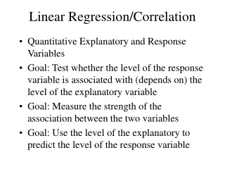
Linear regression and Correlation. Peter Shaw. Introduction. X Y. These inter-related areas together make up one of the most powerful and useful areas of data analysis

Linear regression and Correlation
E N D
Presentation Transcript
Linear regression and Correlation Peter Shaw
Introduction X Y • These inter-related areas together make up one of the most powerful and useful areas of data analysis • They are simple to understand, given a few easily-learnt facts and – crucially – the knack of thinking of data as points in a 2D space. • Do not worry unduly about the formulae or procedures: what matters is the mental imagery. Y X
Y What you need: X • Is 2 variables which are paired together in some way: • Measures against time • Body height vs time: 1 sample per year • Responses to treatments • Growth of plants grown in a series of different fertiliser concentations • One of these is assumed to depend on the other: this is the dependent variable, always shown on the Y axis of a graph • The other is the independent variable, and goes on the X axis. Time, if measured, is always the independent variable – nothing affects the rate of flow of time! X Y Height age
Golden rules for a scattergraph: A graph of yield against fertiliser aplication for this examplar system Label for Y axis = dependent variable Title, which should be fully self-explanatory Draw one best-fit line Plant mass g Label for X axis = independent variable Fertiliser added g
NEVER dot – dot!! Unless your are absolutely sure that interpolation is valid Lichen cover on tombstone This is WRONG year
There are 2 questions you can ask here: X Y • 1: How likely is it that this pattern could occur by chance? • Use correlation • This involves calculating a correlation coefficient r, then finding the probability of obtaining this value of r. • 2: What is the best description of the relationship between the two variables? • Use regression • This involves calculating the equation of the best fit line. • Linear regression tries to explain the relationship as an equation of the form • Y = A + B*X R = 0.95, Df = 8, p < 0.01 Y = 1 + 2*X Y X
Correlation • Here we calculate an index which tells us how closely the data approximate to a straight line • These indices are called correlation coefficients. • There are 2 correlation coefficients, depending on whether the data are normally distributed: • Parametric data: use Pearson’s Product Moment Correlation Coefficient,mercifully always known as r • Non-parametric data: Use Spearman’s correlation Coefficient rs Obscure technical tip: rs is simply r applied to the ranked values of the data
Both correlation coefficients behave in exactly the same way They range between 1.0 and –1.0: never >1 nor <-1 • The value tells you how closely the data approximate to a straight line. r = 0.6 ish r = -1.0 r = 1.0 r = -0.8ish
How to calculate? • 1: You do not need to know this – it is usually done by PC or calculator Non-parametric data: rank X data and Y data separately, find the difference between the X and Y ranks for each observation. Call this difference D then use rs = 1-6*Σ(D*D) _______ (N-1)N(N+1) Parametric data: use r = Σxy - ΣxΣy/N ___________ Sqrt[ (Σxx - ΣxΣx/N) * (Σy*y - ΣyΣy/N) ]
Significance testing: • define your significance level (p=0.05) • H0: There is no association between Y and X: any indication of this is due to chance • H1: There is a relationship between Y and X (which may be +ve or –ve). [WARNING: You are not inferring causality] • Find your df. Here it = N-2 • Compare your r value with the critical value listed in tables – but ignore any negative signs. Larger than tabulated values of r are significant. r = 1.0 Why N-2? Because with 2 data points your line is certain to be a perfect fit
Example data – 2 measures of leaf decomposer activity X = CO2, micL/g/hr • Y = FDA Activity (y)OD/g/hr • X Y • 136.8 40.28 • 72.0 14.46 • 68.4 13.73 • 41.4 8.98 • 91.8 13.73 • 115.2 31.17 • 82.8 23.40 • 161.0 27.94 • 93.6 27.94 r = 0.80, df = 7, p<0.01 rs = 0.86 df =7, p<0.01
Best fit lines • What is meant by a best fit? • There are infinitely many different lines that can be fitted to any dataset, most of which are clearly not a good fit. • There is a formal definition of a best-fit line, and it involves the “residuals”, the deviations of each data point from the best fit line.
A best fit line … • Is the one that minimises the sum of residuals squared. This is known as a least-squares best fit. • The usual best-fit line (supplied by calculators and most PC packages) is the one which minimises the vertical sum of residuals squared for the model • Y = A + B*X Gradient, B, = extent to which Y increases when X increases by 1 Intercept = A =value of Y when X = 0
Be aware that there are alternative models! Usual model: Y = A+B*X with vertical residuals B = Σxy - ΣxΣy/N ___________ Σxx - ΣxΣx/N A = mean(Y) – B*mean(X) Y=B*X, vertical residuals Y = B*X orthogonal residuals Y = A+B*X, orthogonal residuals
Fig 3.6 – The standard model for a best fit line: Residuals are vertical, line passes through the overall mean of the data. The significance of this relationship may be measured by calculating a correlation coefficient. mean value of x, μx mean value of y, μy Dependent variable The gradient of the line may be calculated as follows: B = Σ(X-μx)*(Y-μy) Σ(X-μx)*(X-μx) Intercept = A = μy -B* μx The intercept is generally not zero 0 Independent variable 0
Fig 3.7 – The zero-intercept model for a best fit line: Residuals are vertical, line passes through 0,0. No significance testing or correlation coefficient is possible for this model. Dependent variable Gradient of the line = B = ΣXY ΣXX Intercept = A = 0 The intercept is exactly zero 0 Independent variable 0
Fig 3.8 – The Reduced major axis model for a best fit line: Residuals are orthogonal, the line passes through the overall mean of the data. No significance testing is possible for this model. mean value of x, μx mean value of y, μy Dependent variable Gradient of the line = B = standard deviation (Y) standard deviation (X) Intercept = A = μy -B* μx The intercept is generally not zero 0 Independent variable 0
When you ask for a best-fit line: • What you get are 2 numbers, A and B, the intercept and the gradient. • These are enough to specify the 2 line in 2 dimensional space. • (Note that you can equally fit a best-fit plane in 3D space, but this needs 3 parameters: an intercept and 2 gradients). Why the Y-X choice really matters:
X-Y = Y-X Given 2 variables you can plot 2 equivalent graphs: Y against X, or X against Y. In fact these are not quite the same! Swapping the axes around has no effect on the Correlation (hence the likelihood of the pattern occurring by chance). BUT It does deeply affect the relationship inferred, the actual best fit line. The Y on X line is NOT just the X on Y line transposed. R = -0.9 R = -0.9 IS NOT THE SAME AS: V1 V2 V2 V1
Why “Regression”? The term was coined by Sir Frances Galton in his 1885 address to the BAAS, in describing his findings about the relationship between height of children and of their parents. He found that the heights tended to be to less extreme than their parents – closer to the mean, so tall parents had tall kids, but less extremely tall, while short couples had sort kids, but less extremely short. (The gradient of the Kids on parents line was 0.61) He called this "Regression Towards Mediocrity In Hereditary Stature," (Galton, F. (1886) Inverting this logic might predict that parents are more extreme than heir children. This is not so : the gradient of the parents on kids line was 0.29, even less than the 1.0 expected from equality. Remember: the best fit line does not just transpose when X and Y swap!
This allows us to predict values – an act known as extrapolation Predicted value of Y • Given a regression equation • Y = A + B*X • We can predict the expected value for Y given any value of X. This is exactly equivalent to drawing a line on the graph. Observed value of X
Equation of the regression line: Y = 0.77+0.23*X Correlation coefficient r = 0.80, p<0.01 If the line is constrained to pass through 0,0 its equation becomes Y = 0.23*X. In this case the zero-intercept line is visually indistinguishable from the line plotted. An example:The litter FDA data again 40 When x = 100 Y should be 22.6+0.773 = 23.73 20 FDAactivity, ODg-1 hr-1 50 100 150 CO2, g g-1 hr-1
The DCA ordination of annual toadstool data graphed as a function of year. 0 100 200 1st DCA axis Y = 11.88*X-1003.53 r=0.977 p< 0.001 Year 86 87 88 89 90 91 92 93 94 95 96 97 98 99 00 01
Flowchart for handling regression data Are your data normally distributed? No Yes Calculate r. Is it significant? Calculate Spearman’s correlation coefficient and assess its significance. Consider how best to graph data. Yes No Say you have done the work and it was NS (credit where it’s due!) Plot data and fit a best-fit line. Annotate the graph with r, p and the regression equation.
Reliability • Inter-Rater or Inter-Observer Reliability • Used to assess the degree to which different raters/observers give consistent estimates of the same phenomenon (coefficient of association) • Test-Retest Reliability • Used to assess the consistency of a measure from one time to another (correlation) • Parallel-Forms Reliability • Used to assess the consistency of the results of two tests constructed in the same way from the same content domain (correlation) • Internal Consistency Reliability • Used to assess the consistency of results across items within a test (Cronbach’s alpha).
Cronbach’s alpha This is an index of reliability, and is usually used when comparing a set of questions in a questionnaire score to see whether they genuinely seem to be getting the same sort of results. You will need it to analyse the GHQ data. It is not a statistical test, carries no H0 or significance level, but it does supply a guideline: Cronbach’s alpha >0.7 for a set of questions to be considered reliably consistent. IN SPSS use Scale – reliability analysis, then in save options selected “scale if deleted”. The pattern you want to hunt is of alpha values <0.7 which become >0.7 if one variable is removed; this is warning that the variable is unreliable.