Census 2000 Data Engine Overview: User Guide for DVDs and CD-ROMs
Learn how to use the Census 2000 Data Engine software to select datasets, geographies, and variables for data export and analysis. The guide covers workspace functions, picking geography, output options, simple and custom variables.

Census 2000 Data Engine Overview: User Guide for DVDs and CD-ROMs
E N D
Presentation Transcript
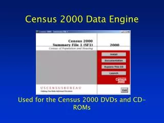
Census 2000 Data Engine Used for the Census 2000 DVDs and CD-ROMs
Software Overview Once the application is launched, the Data Engine screen will appear:
Software Overview, 2 There are five tabs along the top of the workspace. The tabs open pages to walk you through selecting: the dataset, the area(s) of geography, the type of file you want to create, and the data points (variables).
Software Overview, 3 The Back, Next and Finish buttons at the bottom of the box also walk you through the selection process.
Software Overview, 4 The tabs and buttons are available on every screen so you can refine your selections without restarting the Data Engine.
Overview - Workspace The first tab, for the Workspace page, has two functions: Using the Current Database Set menu you can select SF1 or one of the 250 datasets available for racial and ethnic groups using SF2 (if you have both datasets loaded).
Overview, Workspace - 2 The other function of the Workspace page is the ability to save or retrieve a workspace (your selected geography or variables) using the File button. Tip: You’ll want to save your workspace when you plan to reuse geography or variables. This will save time in the future.
Overview, Workspace - 3 The File button, on the Workspace page, allows you to open previously saved workspaces, or to save newly developed ones. Unfortunately, workspaces do not transfer between datasets.
Overview, Pick Geography The next tab, Pick Geography, opens the page for selecting the geographic areas (states, counties, census tracts, blocks, etc.)
Overview, Pick Geography - 2 The File button on this page has three important features. Users may add radii, clear previously used radii, and clear geographic selections.
Overview, Pick Geography - 3 The Custom Radii search allows users datasets based on distance from a point using miles or kilometers.
Overview - Output Tab The Output Taballows users to export data in two ways (modes): • Report, the default option, generates html tables • File exports data into into xls, csv, dbf, htm, mdb and db.
Overview - Simple Variables At the Simple Variables Tab you select data elements (Input Variables).
Overview, Simple Variables - 2 Each dataset has variables divided into several categories, or folders. Roughly, these are • Geographic Identifiers, • H (Housing) Tables, • P (Population) Tables
Overview, Simple Variables - 2 In addition to the P and H tables, there are HCT Tables (Housing Tables to the Census Tract, and PCT Tables (Population Tables to the Census Tract).
Overview, Simple Variables - 3 The Geographic Identifiersdescribe the areas you selected. In SF2 and SF3 these are divided into four categories: • Record Codes, • Geographic Area Codes, • Area Characteristics, and • Special Area Codes. SF1 lists them alphabetically.
Overview, Simple Variables - 4 The other variables, H Tables, P Tables, HCT and PCT tables, are numeric data you may choose for the selected geography.
Overview, Simple Variables - 5 The Input Variables box does not expand in size, however if you “mouse over” the table name, the whole title will appear. Scroll bars may also be used to see titles.
Overview, Simple Variables - 6 As you choose variables (by double-clicking on the variable, or by clicking on the variable and then the Select button) they appear in the Output Variables box.
Overview, Simple Variables - 7 You can select a complete table – including all data items - by highlighting it and clicking on the Select button.
Overview – Custom Variables The Custom Variables page allows users to take simple variables, and as you might in a spreadsheet or database program, perform mathematical functions.
Overview, Custom Variables - 2 By adding, subtracting, multiplying and dividing – creating formulas - new variables are created.
Datasets currently available SF1 provides access to population and housing data based on Census 2000 questions asked of all people and about every housing unit. These data are often referred to as the "100% data."Populationitems include: sex, age, race, Hispanic or Latino origin, household relationship, and household and family characteristics. Housingitems include occupancy status and whether the unit is owner- or renter-occupied (tenure).
Datasets currently available Geographycovered for SF 1 includes: States, counties, county subdivisions, places, census tracts, block groups, blocks, ZIP code tabulation areas, congressional districts (106th Congress), American Indian and Alaska Native Areas, Hawaiian Home Lands.
Datasets currently available SF 2 contains population and housing unit data based on Census 2000 questions asked of all people and about every housing unit (100% data) down to the census tract for 250 population groups.
Datasets currently available Tables are iterated for each of 250 groups - these are the databases for SF 2 listed on the Workspace page: • the total population, • 132 race groups, • 78 American Indian and Alaska Native tribe categories (reflecting 39 individual tribes), and • 39 Hispanic or Latino groups.
Population Threshold In SF2, the presentation of tables for any of the population groups is subject to a population threshold (within any geographic area) of 100 or more people.
Population Threshold -2 After you’ve selected a database, if a census tract or other geographic area doesn’t appear on the Pick Geography page, the population doesn’t meet the 100 threshold. Examples: Two or more races (Group 100) - for Tract 21 in Albuquerque NM; Bangladeshi alone - in 21 states including: AK, AR, HI, ID, IA, ME, MS, MT, NE, NH, NM, ND, RI, SC, SD, UT, VT, WV, WI, WY and PR.
Datasets currently available SF 3 has 813 tables of social, economic, and housing characteristics compiled from approximately 19 million housing units – about 1 in 6 households. Of the 813 tables, 484 are population tables, and 329 are housing tables.
Datasets currently available Geographic Coverage for SF3: Data is presented for the United States, the 50 states, the District of Columbia and Puerto Rico down to the block group for many tabulations, but only to the census tract for others. Summaries are included for other geographic areas, such as ZIP Code Tabulations Areas (ZCTAsTM) and Congressional Districts
Sample Search Go to the Workspace Tab, select SF 1 DVD or SF1 for New Mexico (if you are using the CD-ROM) If another dataset was selected, you may need to wait a minute for the dataset to reload.
Sample Search Move to the next page, Pick Geography. Select all census tracts for a county or place in New Mexico listed below: Places: Albuquerque, Carlsbad, Roswell, Santa Fe, Taos, Truth or Consequences Counties: Bernalillo, Chaves, Eddy, Santa Fe, Sierra, Taos
Sample Search You’ll want to use Summary Level 140 (Census Tract by County) or 158 (Census Tract by County and Place)
Sample Search Click on the “plus box” next to the square to expand the selections. If you click on the empty box, the software will place a checkmark in the box indicating you have selected all of the tracts for the entire country.
Sample Search Next, click on the Output tab. First we’re going to use the default option, Report. For Report, the user chooses from a variety of preformatted reports listed under the Report Template File dropdown menu.
Sample Search Select one of the reports (e.g. DP-1, or Quick Tables P05) and click on the Finish button.
Sample Search A in process note will appear, and then the “processing finished” dialog box, asking if you want to open the output file using the default application, or another application.
Sample Search Below is the output from the tracts for Eddy Co., NM. Note that the county and and state names are not listed, only the Census Tract numbers.
Sample Search Tip: If you are working with multiple numbered areas (tracts or blocks) it is important to note (by keeping records, or by file names) which geographic area they belong to. This applies to named areas, as well. You’ll find many states with county and city names that repeat (e.g. Madison, Franklin, Lincoln, Jefferson, Athens etc.).
Sample Search Close the browser, and return to the Output tab. Click on the Filebutton, then on the Save As button
Sample Search Select the directory, the file name, and the file format for your download. Tip: The “save as” box allows you to save onto the a:\ drive by typing the drive letter.
Sample Search Click on the Simple Variables Tab. Click on the folder to open the Geographic Identifiers.
Sample Search Select (in this order): • State (FIPS) • County • Place (FIPS) • Census Tract • Internal Point (Longitude) • Internal Point (Latitude)
Sample Search Now open any of the other folders and select 3-10 additional data points of your choice. Click on the Finish button.
Sample Search If you are using Excel, the system will ask you if you want to overwrite the file. Click on Yes. Note: The Data Engine software interacts differently with each spreadsheet and database application. Be flexible and try one or two approaches for your own situation if there are problems.
Sample Search Next a dialog box will open to ask if you want to name the worksheet/table. Name it something slightly different (add a letter or number to the end). Click on OK.
Sample Search The “Processing Finished” dialog box will open. Check the box for Open the field descriptions file. Click OK.
Sample Search The spreadsheet software, and the field descriptions file will open.
Sample Search The top row lists the name, several abbreviations for the geographic identifiers, and the codes for the selected simple variables. Note the longitude and latitude for one of your tracts from your output.
Sample Search The Field Description file gives the complete titles for each code and abbreviation used. The Data Engine automatically generates this file, using the same name as the saved file, with a .desc.txt extension


