Recombination and Linkage
Recombination and Linkage. The genetic approach. Start with the phenotype; find genes the influence it. Allelic differences at the genes result in phenotypic differences. Value: Need not know anything in advance. Goal Understanding the disease etiology (e.g., pathways)


Recombination and Linkage
E N D
Presentation Transcript
The genetic approach • Start with the phenotype; find genes the influence it. • Allelic differences at the genes result in phenotypic differences. • Value:Need not know anything in advance. • Goal • Understanding the disease etiology (e.g., pathways) • Identify possible drug targets
Approaches togene mapping • Experimental crosses in model organisms • Linkage analysis in human pedigrees • A few large pedigrees • Many small families (e.g., sibling pairs) • Association analysis in human populations • Isolated populations vs. outbred populations • Candidate genes vs. whole genome
Outline • A bit about experimental crosses • Meiosis, recombination, genetic maps • QTL mapping in experimental crosses • Parametric linkage analysis in humans • Nonparametric linkage analysis in humans • QTL mapping in humans • Association mapping
The data • Phenotypes,yi • Genotypes, xij = AA/AB/BB, at genetic markers • A genetic map, giving the locations of the markers.
Goals • Identify genomic regions (QTLs) that contribute to variation in the trait. • Obtain interval estimates of the QTL locations. • Estimate the effects of the QTLs.
Phenotypes 133 females (NOD B6) (NOD B6)
Statistical structure • Missing data: markers QTL • Model selection: genotypes phenotype
Genetic distance • Genetic distance between two markers (in cM) = Average number of crossovers in the interval in 100 meiotic products • “Intensity” of the crossover point process • Recombination rate varies by • Organism • Sex • Chromosome • Position on chromosome
Crossover interference • Strand choice • Chromatid interference • Spacing • Crossover interference • Positive crossover interference: • Crossovers tend not to occur too • close together.
Recombination fraction We generally do not observe the locations of crossovers; rather, we observe the grandparental origin of DNA at a set of genetic markers. Recombination across an interval indicates an oddnumber of crossovers. Recombination fraction = Pr(recombination in interval) = Pr(odd no. XOs in interval)
Map functions • A map function relates the genetic length of an interval and the recombination fraction. r = M(d) • Map functions are related to crossover interference, but a map function is not sufficient to define the crossover process. • Haldane map function: no crossover interference • Kosambi: similar to the level of interference in humans • Carter-Falconer: similar to the level of interference in mice
Models: recombination • We assume no crossover interference • Locations of breakpoints according to a Poisson process. • Genotypes along chromosome follow a Markov chain. • Clearly wrong, but super convenient.
The simplest method “Marker regression” • Consider a single marker • Split mice into groups according to their genotype at a marker • Do an ANOVA (or t-test) • Repeat for each marker
Marker regression Advantages • Simple • Easily incorporates covariates • Easily extended to more complex models • Doesn’t require a genetic map Disadvantages • Must exclude individuals with missing genotypes data • Imperfect information about QTL location • Suffers in low density scans • Only considers one QTL at a time
Interval mapping Lander and Botstein 1989 • Imagine that there is a single QTL, at position z. • Let qi = genotype of mouse i at the QTL, and assume yi | qi ~ normal( (qi), ) • We won’t know qi, but we can calculate (by an HMM) pig = Pr(qi = g | marker data) • yi, given the marker data, follows a mixture of normal distributions with known mixing proportions (the pig). • Use an EM algorithm to get MLEs of = (AA, AB, BB, ). • Measure the evidence for a QTL via the LODscore, which is the log10 likelihood ratio comparing the hypothesis of a single QTL at position z to the hypothesis of no QTL anywhere.
Interval mapping Advantages • Takes proper account of missing data • Allows examination of positions between markers • Gives improved estimates of QTL effects • Provides pretty graphs Disadvantages • Increased computation time • Requires specialized software • Difficult to generalize • Only considers one QTL at a time
LOD thresholds • To account for the genome-wide search, compare the observed LOD scores to the distribution of the maximum LOD score, genome-wide, that would be obtained if there were no QTL anywhere. • The 95th percentile of this distribution is used as a significance threshold. • Such a threshold may be estimated via permutations (Churchill and Doerge 1994).
Permutation test • Shuffle the phenotypes relative to the genotypes. • Calculate M* = max LOD*, with the shuffled data. • Repeat many times. • LOD threshold = 95th percentile of M*. • P-value = Pr(M* ≥ M)
Going after multiple QTLs • Greater ability to detect QTLs. • Separate linked QTLs. • Learn about interactions between QTLs (epistasis).
Before you do anything… Check data quality • Genetic markers on the correct chromosomes • Markers in the correct order • Identify and resolve likely errors in the genotype data
Software • R/qtl http://www.rqtl.org • Mapmaker/QTL http://www.broad.mit.edu/genome_software • Mapmanager QTX http://www.mapmanager.org/mmQTX.html • QTL Cartographer http://statgen.ncsu.edu/qtlcart/index.php • Multimapper http://www.rni.helsinki.fi/~mjs
Before you do anything… • Verify relationships between individuals • Identify and resolve genotyping errors • Verify marker order, if possible • Look for apparent tight double crossovers, indicative of genotyping errors
Parametric linkage analysis • Assume a specific genetic model. For example: • One disease gene with 2 alleles • Dominant, fully penetrant • Disease allele frequency known to be 1%. • Single-point analysis (aka two-point) • Consider one marker (and the putative disease gene) • = recombination fraction between marker and disease gene • Test H0: = 1/2 vs. Ha: < 1/2 • Multipoint analysis • Consider multiple markers on a chromosome • = location of disease gene on chromosome • Test gene unlinked ( = ) vs. = particular position
Missing data The likelihood now involves a sum over possible parental genotypes, and we need: • Marker allele frequencies • Further assumptions: Hardy-Weinberg and linkage equilibrium
More generally • Simple diallelic disease gene • Alleles d and + with frequencies p and 1-p • Penetrances f0, f1, f2, with fi = Pr(affected | i d alleles) • Possible extensions: • Penetrances vary depending on parental origin of disease allele f1 f1m, f1p • Penetrances vary between people (according to sex, age, or other known covariates) • Multiple disease genes • We assume that the penetrances and disease allele frequencies are known
Likelihood calculations • Define g = complete ordered (aka phase-known) genotypes for all individuals in a family x = observed “phenotype” data (including phenotypes and phase-unknown genotypes, possibly with missing data) • For example: • Goal:
The parts • Prior = Pop(gi) Founding genotype probabilities • Penetrance = Pen(xi | gi) Phenotype given genotype • TransmissionTransmission parent child = Tran(gi | gm(i), gf(i)) Note: If gi = (ui, vi), where ui = haplotype from mom and vi = that from dad Then Tran(gi | gm(i), gf(i)) = Tran(ui | gm(i)) Tran(vi | gf(i))
The likelihood Phenotypes conditionally independent given genotypes F = set of “founding” individuals
That’s a mighty big sum! • With a marker having k alleles and a diallelic disease gene, we have a sum with (2k)2nterms. • Solution: • Take advantage of conditional independence to factor the sum • Elston-Stewart algorithm: Use conditional independence in pedigree • Good for large pedigrees, but blows up with many loci • Lander-Green algorithm: Use conditional independence along chromosome (assuming no crossover interference) • Good for many loci, but blows up in large pedigrees
Ascertainment • We generally select families according to their phenotypes. (For example, we may require at least two affected individuals.) • How does this affect linkage? If the genetic model is known, it doesn’t: we can condition on the observed phenotypes.
Model misspecification • To do parametric linkage analysis, we need to specify: • Penetrances • Disease allele frequency • Marker allele frequencies • Marker order and genetic map (in multipoint analysis) • Question: Effect of misspecification of these things on: • False positive rate • Power to detect a gene • Estimate of (in single-point analysis)
Model misspecification • Misspecification of disease gene parameters (f’s, p) has little effect on the false positive rate. • Misspecification of marker allele frequencies can lead to a greatly increased false positive rate. • Complete genotype data: marker allele freq don’t matter • Incomplete data on the founders: misspecified marker allele frequencies can really screw things up • BAD: using equally likely allele frequencies • BETTER: estimate the allele frequencies with the available data (perhaps even ignoring the relationships between individuals)
Model misspecification • In single-point linkage, the LOD score is relatively robust to misspecification of: • Phenocopy rate • Effect size • Disease allele frequency However, the estimate of is generally too large. • This is less true for multipoint linkage (i.e., multipoint linkage is not robust). • Misspecification of the degree of dominance leads to greatly reduced power.
Other things • Phenotype misclassification (equivalent to misspecifying penetrances) • Pedigree and genotyping errors • Locus heterogeneity • Multiple genes • Map distances (in multipoint analysis), especially if the distances are too small. All lead to: • Estimate of too large • Decreased power • Not much change in the false positive rate Multiple genes generally not too bad as long as you correctly specify the marginal penetrances.