Cost Theory and Estimation
Department of Business Administration. FALL 20 10 - 11. Cost Theory and Estimation. by Ass oc . Prof. Sami Fethi. The Nature of Costs. Explicit Costs Accounting Costs Economic Costs Implicit Costs Alternative or Opportunity Costs Relevant Costs Incremental Costs

Cost Theory and Estimation
E N D
Presentation Transcript
Department of Business Administration FALL 2010-11 Cost Theory and Estimation by Assoc. Prof. Sami Fethi
The Nature of Costs • Explicit Costs • Accounting Costs • Economic Costs • Implicit Costs • Alternative or Opportunity Costs • Relevant Costs • Incremental Costs • Sunk Costs are Irrelevant
The Nature of Costs • Costs are incurred as a result of production. • Economists define cost in terms of opportunities that are sacrificed when a choice is made. Therefore, economic costs are simply benefits lost . • Accountants define cost in terms of resources consumed. Accounting costs reflect changes in stocks (reductions in good things, increases in bad things) over a fixed period of time.
Explicit Costs • Explicit costs are actual expenditures of the firm to hire, rent, or purchase the inputs it requires in production.These includes the wages to hire labor, the rental price of capital, equipment, and buildings, and the purchase price of raw materials and semi finished products.
Implicit Costs • Implicit costs refers to the value of the inputs that are owned and used by the firm in its own production activity. These includes the highest salary that the entrepreneur could earn in his or her best alternative employment and the highest return that the firm could receive from investing its capital in the most rewarding alternative use or renting its land and buildings to the highest bidder.
Economic Costs • Economic cost refers the sum of explicit and implicit costs. These costs must be distinguished from accounting costs, which refer only to the firm’s actual expenditures, or explicit cost, incurred for purchased or hired inputs.
Alternative or Opportunity Costs • The cost to the firm of using a purchased or owned input is equal to what the input could earn in its best alternative use. • The firm must include the alternative or opportunity costs because the firm cannot retain a hired input if it pays a lower price for the input than another firm.
Relevant and Irrelevant Costs • Relevant Costs: The costs that should be considered in making a managerial decision; economic or opportunity costs. • Incremental costs: the total increase in costs for implementing a particular managerial decision. • Irrelevant or Sunk Costs: The cost that are not affected by a particular managerial decision.
Short-Run Cost Functions • In short-run period, some of the firm’s inputs are fixed and some are variable, and this leads to fixed and variable costs. • Total costs is the cost of all the productive resources used by the firm. It can be divided into two separate costs in the short run.
Total fixed and variable costs • Total Fixed Costs: The total obligations of the firm per time period for all the fixed inputs the firm uses. • Total Variable Costs: The total obligations of the firm per time period for all the variable inputs the firm uses.
Short-Run Cost Functions Total Cost = TC = f(Q) Total Fixed Cost = TFC Total Variable Cost = TVC TC = TFC + TVC
Average Costs • Average total cost (also called average cost) equals total cost per unit of output produced ATC = TC/Q • Average fixed cost equals fixed cost divided by quantity produced AFC = FC/Q • Average variable cost equals variable cost divided by quantity produced AVC = VC/Q
Average Costs and Marginal Cost • Average total cost is also the sum of average fixed cost and average variable cost. ATC = AFC + AVC • Marginal (incremental) cost is the increase in total cost resulting from a one-unit increase in output. Marginal decisions are very important in determining profit levels. MC = ΔTC/ΔQ
Average Costs and Marginal Cost • The marginal cost curve, average variable cost curve and average total cost curves are generally U-shaped. • The U-shape in the short run is attributed to increasing and diminishing returns from a fixed-size plant, because the size of the plant is not variable in the short run.
Average Costs and Marginal Cost • The marginal cost and average cost curves are related • When MC exceeds AC, average cost must be rising • When MC is less than AC, average cost must be falling • This relationship explains why marginal cost curves always intersect average cost curves at the minimum of the average cost curve.
MC ATC AVC R TC = ATC* x Q** J TVC = AVC* x Q* Graphical Presentation MC will intersect the AVC at theminimum of the AVC [always]. $ ATC* MC will intersect the ATC at the minimum of the ATC. AVC* The vertical distance betweenATC and AVC at any output isthe AFC. At Q** AFC is RJ. Q** Q* Q At Q* output, the AVC is at a minimum AVC* [also max of APL]. At Q** the ATC is at a MINIMUM.
Relationship Between Marginal and Average Costs If MC > ATC, then ATC is rising If MC = ATC, then ATC is at its minimum If MC < ATC, then ATC is falling If MC > AVC, then AVC is rising If MC = AVC, then AVC is at its minimum If MC < AVC, then AVC is falling
Short-Run Cost Functions Average Total Cost = ATC = TC/Q Average Fixed Cost = AFC = TFC/Q Average Variable Cost = AVC = TVC/Q ATC = AFC + AVC Marginal Cost = TC/Q = TVC/Q
Short-Run Cost Functions-Example Average Total Cost = ATC = TC/Q Average Fixed Cost = AFC = TFC/Q Average Variable Cost = AVC = TVC/Q ATC = AFC + AVC Marginal Cost = TC/Q = TVC/Q
Average Cost Curves-Graphical meaning • The average fixed cost curve slopes down continuously. • The average total cost curve is the vertical summation of the average fixed cost curve and the average variable cost curve • The ATCcurve is always higher than AFC and AVC curves • While output gets big and AFC decline to zero, the AVC curve approaches the ATC curve.
Wage Rate Average Variable Cost AVC = TVC/Q = w/APL Marginal Cost TC/Q = TVC/Q = w/MPL
Long-Run Cost Curves • The long run is the period of time during which: • Technology is constant • All inputs and costs are variable • The firm faces no fixed inputs or costs • The long run period is a series of short run periods. [For each short run period there is a set of TP, AP, MP, MC, AFC, AVC, ATC, TC, TVC & TFC for each possible scale of plant].
Long-Run Cost Curves Long-Run Total Cost = The minimum total costs of producing various levels of output when the firm can build any desired scale of plant: LTC = f(Q) Long-Run Average Cost = The minimum per-unit cost of producing any level of output when the firm can build any desire scale of plant: LAC = LTC/Q Long-Run Marginal Cost = The change in long-run total costs per unit change in output: LMC = LTC/Q
Long-Run Cost Curves Long-Run Total Cost = LTC = f(Q) Long-Run Average Cost = LAC = LTC/Q Long-Run Marginal Cost = LMC = LTC/Q
Derivation of Long-Run Cost Curves From point A on the expansion path in the first panel with w=$ 10 and r=$ 10, the firm uses 4 units of labor 4L and 4 units of capital 4k and the minimum totalcost producing 1Q is $80. This is shown as point A’ and A’’ on the long-run total cost curve in the middle panel and bottom panel.
Relationship Between Long-Run and Short-Run Average Cost Curves The top panel of the figure is based on the assumption that the firm can build only four scales of plant SAC1 etc.., while the bottom panel is based on the assumption that the firm can build many more or an infinite number of scales of plant. At A’’ min av cost of producing o/p is $80. At B* the firm can produce 1.5Q at an av cost of $70 by using either SAC1 or SAC2 and so on..
Possible Shapes of the LAC Curve The left panel shows a U-shaped LAC curve which indicates first decreasing and then increasing returns to scale. The middle panel shows a nearly L-shaped LAC curve which shows that economies of scale quickly give way to constant returns to scale or gently rising LAC. The right panel shows an LAC curve that declines continuously, as in the case of natural monopolies.
Learning Curves The learning curve shows the decline in the average input cost of production with rising cumulative total outputs over time. The learning curve also shows that the average cost is about $ 250 for producing the 100th unit at point F etc..
Learning Curves Average Cost of Unit Q = C = aQb Estimation Form: log C = log a + b Log Q • The Learning curve can be express algebraically as follows: • (C is cost of the Qth unit of output) • ln C = ln a + b ln Q Linearized version, can be easily estimated and interpreted. • ln C = 3 – 0.3 ln Q If Q increases by 1%, then unit (average) costs decrease by 0.3%. Useful to make predictions for the future: how much does the average cost for the 100th unit as well as 200th: • lnC =3 – 0.3ln100 = 2.4 ==> C = antilog of (2.4) =$251.19 • lnC =3 – 0.3ln200 =2.31==>C =antilog of (2.31) =$204.03
Cost-Volume-Profit Analysis Cost-volume-profit or breakeven analysisexamines the relationship among the TR, TC, and total profits of the firm at various levels of o/p. This technique is often used by business executives to determine the sales volume required for the firm to break even and the total profits and losses at other sales levels. The analysis uses a cost-volume-profit chart in which the TR and TC curves are represented by straight lines and the break-even o/p (QB) is determined at their intersection.
Cost-Volume-Profit Analysis The slope of the total revenue TR curve refers to the product price of $10 per unit. The vertical intercept of the total cost of (TC) curve refers TFC of $200, and the slope of the TC curve to the AVC of $5. The break-even with TR=TC $400 at the output (Q) of $40 units per time period at the point B.
Cost-Volume-Profit Analysis Total Revenue = TR = (P)(Q) Total Cost = TC = TFC + (AVC)(Q) Breakeven Volume TR = TC (P)(Q) = TFC + (AVC)(Q) QBE = TFC/(P - AVC)
Break-even o/p QBE = TFC/(P - AVC) P = 40 TFC = 200 AVC = 5 QBE = 40
Operating Leverage and the other concepts Operating leverage: The ratio of the firm’s total fixed costs to its total variable costs. Contribution margin per unit: The excess of the selling price of the product over the average variable costs of the firm (i.e. P-AVC) that can be applied to cover the fixed costs of the firm and to provide profits. Degree of operating leverage (DOL): The percentage change in the firm’s profits divided by the percentage change in output or sales; the sales elasticity of profits.
Operating Leverage Operating Leverage = TFC/TVC Degree of Operating Leverage = DOL
Operating Leverage • The intersection of TR and TC defines the break even quantity of QB=40. With TC’, the break even quantity increases to QB’=45. • TC’ has a higher DOL than TC and therefore a higher QBE
Empirical Estimation Data Collection Issues • Opportunity Costs Must be Extracted from Accounting Cost Data • Costs Must be Apportioned Among Products • Costs Must be Matched to Output Over Time • Costs Must be Corrected for Inflation
Empirical Estimation Functional Form for Short-Run Cost Functions Theoretical Form Linear Approximation
Empirical Estimation Theoretical Form Linear Approximation
Empirical Estimation Long-Run Cost Curves • Cross-Sectional Regression Analysis • Engineering Method • Survival Technique
Empirical Estimation-Example • A computer company wants to estimate the average variable cost fuction of producing hard disks. The firm believes that AVC varies with the level of output and wages. An analyst collects the monthly data over the past two years and deflates the variables using the relevant price indexes. Finally, he regresses TVC fuction on output and wages as follows: • LnTVC=0.14+0.80LnQ+0.036LnW (2.8) (3.8) (3.3) t-values ‾ R²=0.92 DW=1.9 F=125.8
Empirical Estimation-Example • Suppose W= $10, drive the AVC and MC. • What are the shapes of the AVC and MC curves of the firm? • Why did the analyst fit a linear rather than quadratic or cubic TVC function? • Was this application the right choice? Why?
The End Thanks