Modeling Time Series Data
Modeling Time Series Data. Module 5. A Composite Model. We can fit a composite model of the form: Sales = (Trend) * (Seasonality) * (Cyclicality) * (Error). Trend.

Modeling Time Series Data
E N D
Presentation Transcript
Modeling Time Series Data Module 5
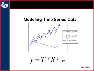
A Composite Model We can fit a composite model of the form: Sales = (Trend) * (Seasonality) * (Cyclicality) * (Error)
Trend Trend is the long term level and the pattern of change in the dependent variable. It is estimated as a simple function of the period number (time). Linear regression or method of least squares is used to estimate the trend. A linear model captures the general upward (or downward) trend with steady growth.
Seasonality Seasonality is a cycle with a period of exactly one year. We estimate it as a proportion of trend for each season. Data must be available on seasonal basis. Time series decomposition is a method to estimate seasonal component. Seasonality captures regular, predictable deviations from the trend. Typical seasons are quarters, weeks, or days.
Cyclicality Cyclicality captures the effects of long-term macroeconomic boom-bust cycles. It is often difficult to get enough data to measure accurately.
Composite Model Any residual deviations are attributed to random error.
Time Series Decomposition • Start with raw data (y) • Estimate Seasonal Indices • Compute base trend using centered moving averages (t’) • Estimate seasonal ratios (y/t’) • Average seasonal ratios to get raw seasonal indices • Normalize seasonal indices (s) • De-seasonalize the raw data (y/s) • Estimate the trend equation using de-seasonalized data (t) • Forecast y’ = t * s • Calculate error = y – (t*s)
Example: Modeling Trend and Seasonality Toys R Us Revenue (millions $)
Example: Computing Moving Averages Calculate Moving Average with span of 4 (1026 + 1056 + 1182 + 2861) 4 = 1531.3
Example: Using centered moving averages to estimate base demand Center Moving Average if using even number of data points (1531.3 + 1567.8) 2 = 1549.5
Example: Computing Seasonal Ratios Calculate the ratio of the revenue to the centered moving average 1182 1549.5 = .7628
Example: Calculating raw Seasonal Indices Calculate the average ratio for each season (quarter). .7162 + .6949 + .7006 + .7424 4 Raw Seasonal Index = .7135
Example: Normalizing Seasonal Indices Normalize to make sure Seasonal Indices average to 1.0 (or add up to 4 in this case) .7135 . .7135+.7077+.7406+1.844 = .7124
Example: De-Seasonalizing raw data Deseasonalize observations. 1026 .7124 = 1440.2 y’ = y/s
Example: De-Seasonalizing Fit a regression line to the deseasonalized observations – y’ (using time as the independent variable).
Example: De-Seasonalizing 56.93 * (1) + 1373.4 = 1430.3 Use trend to make deseasonalized predictions - T
Example: De-Seasonalizing 2568.9 * .71241 = 1830.2 Reseasonalize predictions (T*S)to make forecasts into the future.
Example: De-Seasonalizing Plot the forecasts – T*S
Example: De-Seasonalizing (1026 – 1018.98) 2 = 97.0 As an alternative goodness of fit measure, calculate Root Mean Square Error. RMSE = 9865.2 = 99.3 Average square error
Example: De-Seasonalizing with Statpro http://www.indiana.edu/~mgtsci/StatPro.html Statpro can be used to calculate seasonal indices. Click on Statpro -> Forecast.
Example: De-Seasonalizing with Statpro Select the dependent variable.
Example: De-Seasonalizing with Statpro Select quarterly data.
Example: De-Seasonalizing with Statpro Select a span of 4 and a moving average method of deseasonalizing.
Example: De-Seasonalizing with Statpro Statpro generates the same values that we calculated manually. (Statpro output)

