Download
1 / 24
240 likes | 343 Vues
Explore the methodology of enrollment forecasting through time series modeling, regression analysis, and exponential smoothing techniques. Learn how to predict enrollments based on factors like population, tuition, and past trends for accurate projections. Discover the benefits of incorporating seasonal patterns and trend components in forecasting models. Improve your predictive accuracy and make informed decisions for budgeting and planning in educational institutions.

E N D
Using Time Series Modeling to Forecast Enrollments Robert J. Marsh, Ph.D. Associate Dean of Research and Assessment North Central Michigan College MI/AIR, November 8, 2013
Why forecast enrollment? • Declining enrollment since 2010 • Declining property tax base • Declining state appropriation • Uncertain budgeting process due to lack of data • ACCURATE FORECASTS ARE MORE IMPORTANT THAN EVER
Previous forecasts • Intuitive, sense of potential population • Trends in HS graduations • Conversations with HS counselors • Conversations with workforce organizations and advisory boards • Assume flat enrollment for budget; be pleased with an increase • Assume a 2-3% year-over-year increase • Held steady for many years • Extrapolate from recent terms’ trend • Monitor statewide trends among CCs • No data-informed methodology
An enrollment forecast model • Possible factors • Area population • Tuition • Area unemployment • High school graduate census • Past enrollments • Competition, especially online • Tuition differential, four-year vs. community college • Attitude towards education in general • Community colleges in particular
Regression approach • Identify factors (xi), find coefficients (bi) • Identifying relevant or interesting (or pertinent) factors • Enrollments can be more dependent on past enrollments than outside factors
Area population • Sometimes highly correlated, but not always. Pop change ~ 2% CH change ~ 26%
Time series forecasting • Relies on past demand to forecast future • Stores only one past period’s demand (originally necessary) • Typically forecasts one period ahead
Time series forecasting • Simple: forecast = immediate past period • Moving average: average of n past periods
Exponential Smoothing • Originated in the production/operations management field, 50+ years ago (management science) • Primary formula where a is the “smoothing coefficient” • Relies on the past period’s actual (At-1) and forecast (Ft-1) values. • An a close to 1.0 results in a very reactive model, one more responsive to very recent actual data. • All that needed to be stored were the immediate past actual and forecast values. (Holt, 1957)
Exponential Smoothing • Each period’s forecast builds on all past periods, although only immediate past period’s needs to be stored
“Exponential” Smoothing • Reliance on progressively older data drops off exponentially
Exponential Smoothing with trend • Trends within our actual enrollment patterns. • Add a trend component where b is the “trend factor” (Holt & Winters, 1960; Hopp& Spearman, 2011)
Seasonality • Enrollment is seasonal, with fall typically being higher than winter • Add a seasonality factor by superimposing a sinusoidal function • Exclude summers (much lower) Fall Winter
Seasonality • Sine function is periodic over 2p, every two periods (every fall) the forecast tends to be higher. (Middleton, 2010)
Methodology • Obtained 30 years of enrollment data (credit hours) • 60 periods (no summers) • Built model in Excel® 2011 • Used Solver®to “optimize” the model • Minimized sum of squared differences (the objective function, Z) by varying a, b, H, nand f
Excel®-spreadsheet Parameters
Excel®-Solver® Z a, b, H, n, f a b f
Results • Initially used actual data through Winter 2011-12 to forecast Fall 2012-13 • Discovered strong “starting point dependency” within the non-linear model in Solver • Not optimal; best described as heuristic Results through Winter 2011-12, showing “best”: MAPE = 3.3%. Using model would have produced a 1.7% error for W12 *
Results • Used “best” from W12 to forecast Fall 2012 • F12 forecast = 21,980 • F12 actual = 21,878 • Difference = 0.5% • Model MAPE = 3.3% • Incorporated actual F12 data into model to forecast Winter 2013 *
Results • Used “best” from F12 to forecast Winter 2013 • W13 forecast = 19,783 • W13 actual = 21,081 • Difference = – 6.2% • Model MAPE = 3.4% • Resulted in an under-forecast • Assumes past practices continue • More focused recruitment effort made
Discussion • Model is not optimal • Non linear objective function; heuristic methodology • Does not include any outside variables (as written) • Solver® is blunt instrument • Can be built on simple software platform • Good visualization with graphs • Relies on known data • Very quick to update and do what-if analysis • Pretty accurate
I’m happy to share Bob Marsh North Central Michigan College 231.439.6353 rmarsh@ncmich.edu