Download
1 / 73
730 likes | 886 Vues
Let It Rain: Modeling Multivariate Rain Time Series Using Hidden Markov Models. Sergey Kirshner Donald Bren School of Information and Computer Sciences UC Irvine. March 2, 2006. Acknowledgements. Padhraic Smyth UCI. Andy Robertson IRI. DOE (DE-FG02-02ER63413).

E N D
Let It Rain: Modeling Multivariate Rain Time Series Using Hidden Markov Models Sergey Kirshner Donald Bren School of Information and Computer Sciences UC Irvine March 2, 2006
Acknowledgements Padhraic Smyth UCI Andy Robertson IRI DOE (DE-FG02-02ER63413)
http://iri.columbia.edu/climate/forecast/net_asmt/2006/feb2006/MAM06_World_pcp.htmlhttp://iri.columbia.edu/climate/forecast/net_asmt/2006/feb2006/MAM06_World_pcp.html
What to Do with Rainfall Data? Description historical rainfall data model general circulation model (GCM) outputs
What to Do with Rainfall Data? Downscaling historical rainfall data predicted data model general circulation model (GCM) outputs
What to Do with Rainfall Data? Simulation crop modeling historical rainfall data predicted data model general circulation model (GCM) outputs water management
Modeling Precipitation Occurrence… Northeast Brazil 1975-2002 (except 1976, 78, 84, and 86) 24 seasons (N) 90 days (T) 10 stations (M)
Spell Run Length Distributions Dry spells are in blue; wet spells are in red.
Important Data Characteristics • Correlation • Spatial dependence • Temporal structure • Run-length distributions • Persistence • First order dependence • Variability of individual series • Interannual variability: important for climate studies
Missing Data Missing data mask (black) for 41 stations (y-axis) in India for May 1 - Oct 31, 1973. 29% of the data is missing, with stations 13 14, 16, 24, 26, 30, 36, 38, and 40 missing more than 45% of the data for that station.
A Bit of Notation • Vector time series R • Vector observation of R at time t R11 R21 RT1 R12 R22 RT2 R13 R23 RT3 R1M R2M RTM R1 R2 RT
R1 R2 RT R11 R21 RT1 R12 R22 RT2 R13 R23 RT3 R1M R2M RTM R1 R2 RT Weather Generator • Does not take spatial correlation into account
day 1 day 2 day 3 day T R1 R2 R3 RT Rain Generating Process
R1 R2 Rt RT-1 RT S1 S2 St ST-1 ST Hidden Markov Model (HMM) • Discrete weather states S (K states) • Evolution of the weather state – transition probability P(St|St-1) • Rainfall generation in weather state i – emission probability P(Rt|St=i)
Hidden Markov Model (HMM) R1 R2 Rt RT-1 RT S1 S2 St ST-1 ST
R1 R2 Rt RT-1 RT S1 S2 St ST-1 ST Basic Operations with HMMs • Probability of weather states given observed data (inference) • Forward-Backward • Model parameter estimation given the data • Baum-Welch (EM) • Most likely sequence of weather states given the data • Viterbi [Rabiner 89]
States for 4-state HMM [Robertson, Kirshner, Smyth 04]
Weather State Evolution [Robertson, Kirshner, and Smyth 04]
R1 R2 Rt RT-1 RT S1 S2 St ST-1 ST Generalizations to HMMs: Auto-regressive HMM (AR-HMM) • Explicitly models temporal first-order dependence of rainfall
R1 R2 Rt RT-1 RT S1 S2 St ST-1 ST X1 X2 Xt XT-1 XT Generalizations to HMMs: Non-homogeneous HMM (NHMM) • Incorporates atmospheric variables • Allows non-stationary and oscillatory behavior [Hughes and Guttorp 94; Bengio and Frasconi 95]
Parameter Estimation • Find Qmaximizing P(r|Q) (ML) or P(Q|r) (MAP) • Cannot be done in closed form • EM (Baum-Welch for HMMs) • E-step: compute • Forward-Backward • Calculate • M-step: • Maximize • Can be split into maximization of emission and transition parameters:
Modeling Approaches • Use HMMs • Transition probabilities for temporal dependence • Emissions (hidden state distributions) for spatial or multivariate dependence (and additional temporal dependence) • Emphasis on categorical valued data • Transitions and emissions can be specified separately • Covers cross-product of models
Modeling Approaches (cont’d) • Use HMMs • Possible emission distributions • Conditional independence • Chow-Liu trees [Chow and Liu 68], conditional Chow-Liu forests [Kirshner et al 04] • Markov Random Fields • Maximum entropy models [e.g., Jelinek 98], Boltzmann machines [e.g., Hinton and Sejnowski 86], thin junction trees [Bach and Jordan 02] • Belief Networks • Sigmoidal belief networks[Neal 92] • Possible transition distributions • Non-homogeneous mixture (mixture of experts [Jordan and Jacobs 94]) • Stationary transition matrix • Non-homogeneous transition matrix ([Hughes and Guttorp 94, Meila and Jordan 96, Bengio and Fasconi 95])
Rt1 Rt3 Rt Rt2 RtM = St St HMM-CI [e.g., Zucchini and Guttorp 91; Hughes and Guttorp 94]
Why Use HMM-CI? • Simple and efficient • O(TKM) for inference and for parameter estimation • Small number of free parameters • Can handle missing data • Can be used to model amounts
Rt1 Rt2 Rt3 RtM Rt Ot1 Ot2 Ot3 OtM = St St HMM-CI for Amounts • Types of mixture components • Gamma [Bellone 01] • Exponentials [Robertson et al 06]
Why not HMM-CI • Not matching spatial correlations or persistence well • Models spatial correlation implicitly through hidden states • May require large K to model regions with moderate number of stations
Rt1 Rt3 Rt Rt2 RtM = St St HMM-Autologistic [Hughes, Guttorp, and Charles 99]
Sure! Models spatial correlations very well Can use sampling or approximate schemes to compute normalization constant and to update parameters Not so sure Complexity of exact computation is exponential in M What about temporal dependence? May have too many free parameters if not constrained Does not handle missing values (or very slow) What about HMM-Autologistic?
Neither Here nor There • HMM-CI efficient but too simplistic • HMM-Autologistic more capable but computationally more cumbersome • Want something in between • Computationally tractable • Emission spatial dependence • Additional temporal dependence • Missing values
Bayesian Networks and Trees • Tree-structured distributions • Chow-Liu trees (spatial dependence) [Chow and Liu 68] • With HMMs [Kirshner et al 04] • Conditional Chow-Liu forests (spatial and temporal dependence) [Kirshner et al 04] • Markov (undirected) and Bayesian (directed) networks • MaxEnt (logistic) • Conditional MaxEnt • Sigmoidal belief networks [Neal 92] • Would need to estimate both the parameters and the structure
Chow-Liu Trees • Approximation of a joint distribution with a tree-structured distribution[Chow and Liu 68] • Maximizing log-likelihood solving maximum spanning tree (MST) problem • Can find both the tree structure and the parameters in one swoop! • Finding MST is quadratic in the number of nodes [Kruskal 59] • Edge weights are pairwise mutual information values – measure of conditional independence
B D A B D A C B D A C C AB AC AD BC BD CD Pmarginal (A,B) Pmarginal (A,C) Pmarginal (A,D) Pmarginal (B,C) Pmarginal (B,D) Pmarginal (C,D) Pmarginal (A,B) Pmarginal (A,C) Pmarginal (A,D) Pmarginal (B,C) Pmarginal (B,D) Pmarginal (C,D) AB AC AD BC BD CD 0.3126 0.0229 0.0172 0.0230 0.0183 0.2603 Learning Chow-Liu Trees 0.3126 0.0229 0.0172 0.0230 0.0183 0.2603
Chow-Liu Trees • Approximation of a joint distribution with a tree-structured distribution[Chow and Liu 68] • Properties • Efficient: • O(TM2B2) • Optimal • Can handle missing data • Mixture of trees[Meila and Jordan 00] • More expressive than trees yet with simple estimation procedure • HMMs with trees[Kirshner et al 04]
R1 R2 Rt RT-1 RT S1 S2 St ST-1 ST Rt1 Rt2 Rt1 Rt2 Rt1 Rt2 Rt Rt3 Rt4 Rt3 Rt4 Rt3 Rt4 = St=1 St=2 St=3 St St HMM-Chow-Liu [Kirshner et al 04]
Rt1 Rt2 Rt1 Rt2 Rt1 Rt2 Rt Rt3 Rt4 Rt3 Rt4 Rt3 Rt4 = St=1 St=2 St=3 St St Tree-structured Emissions for Amounts Ot1 Ot2 Rt1 Rt2 Ot3 Ot4 Rt3 Rt4 St=1
Improving on Chow-Liu Trees • Tree edges with low MI add little to the approximation. • Observations from the previous time point can be more relevant than from the current one. • Idea: Build Chow-Liu tree allowing it to include variables from the current and the previous time point.
Conditional Chow-Liu Forests • Extension of Chow-Liu trees to conditional distributions • Approximation of conditional multivariate distribution with a tree-structured distribution • Uses MI to build maximum spanning (directed) trees (forest) • Variables of two consecutive time points as nodes • All nodes corresponding to the earlier time point considered connected before the tree construction • Same asymptotic complexity as Chow-Liu trees • Optimal (within the class of structures) [Kirshner et al 04]
C’ C’ C’ A’ A’ B’ B’ A’ B’ AB AC BC A’A A’B A’C B’A B’B B’C C’A C’B C’C AB AC BC A’A A’B A’C B’A B’B B’C C’A C’B C’C Pmarginal (A,B) Pmarginal (A,C) Pmarginal (B,C) Pmarginal (A’,A) Pmarginal (A’,B) Pmarginal (A’,C) Pmarginal (B’,A) Pmarginal (B’,B) Pmarginal (B’,C) Pmarginal (C’,A) Pmarginal (C’,B) Pmarginal (C’,C) Pmarginal (A,B) Pmarginal (A,C) Pmarginal (B,C) Pmarginal (A’,A) Pmarginal (A’,B) Pmarginal (A’,C) Pmarginal (B’,A) Pmarginal (B’,B) Pmarginal (B’,C) Pmarginal (C’,A) Pmarginal (C’,B) Pmarginal (C’,C) 0.3126 0.0229 0.0230 0.1207 0.1253 0.0623 0.1392 0.1700 0.0559 0.0033 0.0030 0.0625 B A C A A C B B A B C C C’ A’ B’ Example of CCL-Forest Learning 0.3126 0.0229 0.0230 0.1207 0.1253 0.0623 0.1392 0.1700 0.0559 0.0033 0.0030 0.0625
R1 R2 Rt-1 Rt RT S1 S2 St-1 St ST Rt-11 Rt-11 Rt-11 Rt1 Rt2 Rt1 Rt2 Rt1 Rt2 Rt-12 Rt-12 Rt-12 Rt-1 Rt Rt-13 Rt-13 Rt-13 Rt4 Rt3 Rt4 Rt3 Rt4 Rt3 Rt-14 Rt-14 Rt-14 St St HMM-Conditional-Chow-Liu = St=1 St=2 St=3 [Kirshner et al 04]
Beyond Trees • Can learn more complex structure • Optimality not guaranteed [Chickering 96; Srebro 03] • Structure and parameters may have to be learned in separate computations • Computationally expensive • Independence model matches all univariate marginals • Chow-Liu trees match all univariate and some bivariate marginals • Unconstrained Bayesian or Markov Networks • May have too few data points for the number of parameters • Even 3rd order cliques may have zero probability mass
Log-linear or Logistic a b c d
Maximum Entropy Method • Given • Target distribution (empirical) • Set of features and corresponding constraints • Example: feature is 1 when it rains both at station 1 and 2 • Corresponding constraint • Interpretation • Proportion of time it rains simultaneously at stations 1 and 2 is the same for both the historical data and according to the learned distribution • Want to satisfy all of the constraints [e.g., Jelinek 98]
MaxEnt Method (cont’d) • Maximize entropy of subject to constraints corresponding to features • Exponential form • satisfying all of the constraints for features in maximizes the log-likelihood of the data!!! [e.g., Della Pietra et al 97] • Such solution is unique (likelihood is concave)
Rt1 Rt3 Rt Rt2 RtM = St St HMM-Autologistic [Hughes, Guttorp, and Charles 99]
Conditional Log-linear Distribution a d b e c